
Bitcoin Cycles Part 2: The Bottom Signals Are Aligning — Why I'm Starting to DCA
A follow-up to Bitcoin Cycles: A Quantitative Analysis of Halving Events and Price Dynamic

A follow-up to Bitcoin Cycles: A Quantitative Analysis of Halving Events and Price Dynamic
Where We Left Off
In Part 1, we were 20 months post-halving and 2 months past the October 2025 cycle peak of $126,210, trading around $90,000. The forecast for 2026 was explicit:
“Q2-Q3 2026: Potential bear market begins. Historical analogs suggest $50,000-$70,000 possible... Q4 2026-2027: Bear market bottom formation.”
As of July 5, 2026, Bitcoin is trading at $62,718 — down roughly 50% from the October 2025 ATH, and already inside the $50K-$70K zone flagged back in Part 1, ahead of the original “Q4 2026” timeline. That’s the trigger for this post: the bear market arrived faster than the base case, and it’s worth checking, with real numbers, whether the setup here looks more like an accumulation zone or a mid-drawdown trap.
Pulling Fresh Data
import yfinance as yf
import pandas as pd
import numpy as np
from datetime import timedelta

btc = yf.download('BTC-USD', start='2014-09-17', auto_adjust=False, progress=False)

if isinstance(btc.columns, pd.MultiIndex):
    btc.columns = btc.columns.droplevel(1)

btc = btc[['Close']].copy()
btc = btc[~btc.index.duplicated(keep='last')]

print(f"Data range: {btc.index.min().date()} to {btc.index.max().date()}")
print(f"Rows: {len(btc)}")
Data range: 2014-09-17 to 2026-07-05
Rows: 4310Mayer Multiple and Pi Cycle
Two indicators do a lot of work in this post, so it’s worth being precise about what they actually measure before running the numbers.
Mayer Multiple is about as simple as valuation metrics get: current price divided by the 200-day moving average. Above 1.0, price is running hot relative to its own recent trend; below 1.0, it’s trading beneath it. Trace Mayer’s own backtesting on this found that consistently buying whenever the multiple sat below 2.4 produced the best long-run outcomes, and the deepest, most reliable accumulation windows have historically shown up below 1.0 — sometimes dropping as low as 0.5-0.6 in the depths of a bear market. Above 2.4 has marked speculative-bubble territory at every major cycle top (2013, 2017, 2021). It’s a blunt instrument — pure price trend, nothing else — but that’s also what makes it hard to argue with.
Pi Cycle Top is a different kind of signal: it compares the 111-day moving average to 2x the 350-day moving average. When the shorter-term average crosses above that line, it’s flagged nearly every major Bitcoin cycle top with uncanny precision historically. The distance between the two tells you how far price is from that kind of blow-off top condition — a large negative distance means the 111-day average is nowhere near crossing, which is exactly the opposite of what a euphoric, toppy market looks like.
Together they answer two different questions: Mayer Multiple asks “is price cheap or expensive relative to its own recent history,” while Pi Cycle asks “does this look like the kind of parabolic move that’s marked past tops.” Running both against today’s data:
btc['MA_200'] = btc['Close'].rolling(200).mean()
btc['Mayer_Multiple'] = btc['Close'] / btc['MA_200']
btc['MA_111'] = btc['Close'].rolling(111).mean()
btc['MA_350_x2'] = btc['Close'].rolling(350).mean() * 2

latest = btc.dropna(subset=['Mayer_Multiple']).iloc[-1]
latest_date = latest.name

print(f"=== Latest available reading: {latest_date.date()} ===")
print(f"Close:            ${latest['Close']:,.0f}")
print(f"200-day MA:       ${latest['MA_200']:,.0f}")
print(f"Mayer Multiple:   {latest['Mayer_Multiple']:.2f}")
pi_distance = (latest['MA_111'] / latest['MA_350_x2'] - 1) * 100
print(f"Pi Cycle distance: {pi_distance:.1f}% ({'TOP SIGNAL' if pi_distance > 0 else 'no signal'})")
=== Latest available reading: 2026-07-05 ===
Close: $62,718
200-day MA: $74,709
Mayer Multiple: 0.84
Pi Cycle distance: -60.2% (no signal)A Mayer Multiple of 0.84 means price is trading 16% below its own 200-day trend. Per Trace Mayer’s original backtests, accumulating whenever the multiple sits below 1.0 has historically produced the best long-run entries — the long-term average sits around 1.4-1.5, and readings below 0.8 have historically shown up during extended bear markets, not near tops. Pi Cycle isn’t remotely close to a top signal, which is exactly what you’d expect this far into a drawdown.
Re-Running the Strategy Class
Part 1 defined cycle_position_sizing(), risk_adjusted_positioning(), and a BitcoinCycleStrategy class. Running that same logic on today’s numbers:
def cycle_position_sizing(days_from_halving, days_from_peak=None, base_position=1.0):
    if days_from_peak is not None and days_from_peak > 0:
        if days_from_peak <= 90:
            return base_position * 0.5
        elif days_from_peak <= 180:
            return base_position * 0.3
        elif days_from_peak <= 365:
            return base_position * 0.2
        else:
            return base_position * 0.1
    if days_from_halving < 0:
        return base_position * 0.75
    elif 0 <= days_from_halving < 200:
        return base_position * 1.0
    elif 200 <= days_from_halving < 400:
        return base_position * 1.25
    elif 400 <= days_from_halving < 547:
        return base_position * 0.75
    else:
        return base_position * 0.25

def risk_adjusted_positioning(current_price, ma_200, mayer_multiple):
    risk_score = 1.0
    risk_score *= 1.2 if current_price > ma_200 else 0.6
    if mayer_multiple < 1.0:
        risk_score *= 1.3
    elif mayer_multiple <= 2.0:
        risk_score *= 1.0
    elif mayer_multiple <= 2.4:
        risk_score *= 0.7
    else:
        risk_score *= 0.3
    return min(risk_score, 1.5)

class BitcoinCycleStrategy:
    def __init__(self, base_allocation=1.0):
        self.base_allocation = base_allocation
        self.current_halving = pd.to_datetime('2024-04-20')
        self.cycle_peak = pd.to_datetime('2025-10-06')

    def get_cycle_phase(self, current_date):
        days_from_halving = (current_date - self.current_halving).days
        days_from_peak = (current_date - self.cycle_peak).days
        if days_from_peak > 0:
            return ('EARLY_POST_PEAK' if days_from_peak <= 90 else
                    'DISTRIBUTION' if days_from_peak <= 365 else 'BEAR_MARKET')
        return ('PRE_HALVING' if days_from_halving < 0 else
                'EARLY_CYCLE' if days_from_halving < 200 else
                'MID_CYCLE' if days_from_halving < 400 else 'LATE_CYCLE')

    def generate_signal(self, current_date, current_price, ma_200, mayer_multiple):
        days_from_halving = (current_date - self.current_halving).days
        days_from_peak = (current_date - self.cycle_peak).days if current_date > self.cycle_peak else None
        cycle_mult = cycle_position_sizing(days_from_halving, days_from_peak, self.base_allocation)
        risk_mult = risk_adjusted_positioning(current_price, ma_200, mayer_multiple)
        final_position = cycle_mult * risk_mult
        signal = ('ACCUMULATE' if final_position > 0.8 else
                  'HOLD' if final_position > 0.5 else
                  'REDUCE' if final_position > 0.3 else 'DEFENSIVE')
        return signal, {
            'phase': self.get_cycle_phase(current_date),
            'cycle_multiplier': cycle_mult, 'risk_multiplier': risk_mult,
            'final_position': final_position,
            'days_from_halving': days_from_halving,
            'days_from_peak': days_from_peak if days_from_peak else 'N/A',
        }

strategy = BitcoinCycleStrategy(base_allocation=1.0)
signal, position_data = strategy.generate_signal(
    latest_date, latest['Close'], latest['MA_200'], latest['Mayer_Multiple']
)

print(f"=== STRATEGY SIGNAL ({latest_date.date()}) ===")
print(f"Signal: {signal}")
print(f"Phase: {position_data['phase']}")
print(f"Days from halving: {position_data['days_from_halving']}")
print(f"Days from peak: {position_data['days_from_peak']}")
print(f"Cycle multiplier: {position_data['cycle_multiplier']:.2f}x")
print(f"Risk multiplier: {position_data['risk_multiplier']:.2f}x")
print(f"Final position: {position_data['final_position']:.2f}x base allocation")
=== STRATEGY SIGNAL (2026-07-05) ===
Signal: DEFENSIVE
Phase: DISTRIBUTION
Days from halving: 806
Days from peak: 272
Cycle multiplier: 0.20x
Risk multiplier: 0.78x
Final position: 0.16x base allocationThis is worth sitting with rather than talking past: at 272 days past the October 2025 peak, the calendar overlay is still deep in its most defensive bracket, and the trend-following risk overlay agrees — price ($62,718) is still well below its 200-day MA ($74,709), so that factor drags the risk multiplier to 0.6x before the sub-1.0 Mayer Multiple partially offsets it to 0.78x. Both halves of the Part 1 model currently say defensive, not accumulate. That’s the honest starting point for everything below.
Does Buying ~270 Days Post-Peak Actually Work?
Instead of asserting that buying into a drawdown works, it’s worth checking what happened the last two times Bitcoin was roughly this far past a cycle peak:
def backtest_entry_window(prices: pd.Series, entry_date: str, hold_days: int = 365, weekly_budget: float = 100.0):
    entry = pd.to_datetime(entry_date)
    window = prices[(prices.index >= entry) & (prices.index <= entry + timedelta(days=hold_days))]
    weekly = window.resample('W').last().dropna()

    dca_btc = (weekly_budget / weekly).sum()
    dca_cost = weekly_budget * len(weekly)
    lumpsum_btc = dca_cost / weekly.iloc[0]
    final_price = weekly.iloc[-1]

    return {
        'entry_date': entry_date, 'end_date': weekly.index[-1].date(), 'weeks': len(weekly),
        'start_price': weekly.iloc[0], 'end_price': final_price,
        'dca_return_pct': (dca_btc * final_price / dca_cost - 1) * 100,
        'lumpsum_return_pct': (lumpsum_btc * final_price / dca_cost - 1) * 100,
    }

# 2018 cycle: ~270 days past the Dec 2017 peak lands mid-September 2018
# 2022 cycle: ~270 days past the Nov 2021 peak lands mid-August 2022
for entry in ['2018-09-15', '2022-08-15']:
    r = backtest_entry_window(btc['Close'], entry, hold_days=365)
    print(f"Entry {r['entry_date']} -> {r['end_date']} ({r['weeks']} weeks)")
    print(f"  Start: ${r['start_price']:,.0f}  End: ${r['end_price']:,.0f}")
    print(f"  DCA return:      {r['dca_return_pct']:+.1f}%")
    print(f"  Lump-sum return: {r['lumpsum_return_pct']:+.1f}%\n")
Entry 2018-09-15 -> 2019-09-15 (53 weeks)
Start: $6,517 End: $10,348
DCA return: +85.2%
Lump-sum return: +58.8%
Entry 2022-08-15 -> 2023-08-20 (53 weeks)
Start: $21,534 End: $29,170
DCA return: +28.9%
Lump-sum return: +35.5%Mixed results, and that’s worth reporting honestly rather than cherry-picking. In 2018, DCA won because price fell hard again (toward $3,200 that December) before recovering, so spreading purchases across the window captured the lower prices. In 2022, price climbed steadily off the low without a second leg down, so lump-sum captured more of the upside by being fully invested earlier. Two data points isn’t a statistically robust sample — but it’s a clear demonstration that “buy the ~270-day-post-peak zone” has, twice now, sat closer to the accumulation phase than the euphoria phase, with the DCA-vs-lump-sum edge depending entirely on whether there’s a second drawdown leg, which is never knowable in advance.
What Price Alone Can’t Tell You
Mayer Multiple and Pi Cycle only need price data. MVRV-Z Score and the Fear & Greed Index need on-chain and sentiment data instead, so they’re sourced from public trackers (bitbo.io, alternative.me) rather than computed here:
def onchain_value_score(mayer_multiple, mvrv_z, fear_greed):
    """Composite accumulation score, [0,1], higher = more attractive."""
    mayer_score = 1.0 if mayer_multiple < 1.0 else max(0, 1 - (mayer_multiple - 1.0) / 1.4)
    mvrv_score = max(0, 1 - abs(mvrv_z) / 2.0)
    fg_score = max(0, (30 - fear_greed) / 30) if fear_greed < 30 else 0
    weights = {'mayer': 0.4, 'mvrv': 0.35, 'fg': 0.25}
    composite = mayer_score * weights['mayer'] + mvrv_score * weights['mvrv'] + fg_score * weights['fg']
    return composite, {'mayer_score': mayer_score, 'mvrv_score': mvrv_score, 'fg_score': fg_score}

# Mayer Multiple: computed above (0.84, July 5, 2026)
# MVRV-Z and Fear/Greed: public trackers, early July 2026
score, parts = onchain_value_score(mayer_multiple=0.84, mvrv_z=0.20, fear_greed=18)
print("sub-scores:", parts)
print("composite:", round(score, 2))
sub-scores: {'mayer_score': 1.0, 'mvrv_score': 0.9, 'fg_score': 0.4}
composite: 0.82A composite score of 0.82 is high — but two of its three inputs come from external trackers rather than a reproducible calculation, so it’s directional context, not a hard number with the same footing as the backtest above.
A Second, Independent Read: My Price-Prediction Model
Everything above comes from price-derived and on-chain-style metrics. It’s worth checking against a completely different methodology, so here’s what one of my ML forecasting models (same family as the LSTM/GRU/hybrid work covered elsewhere on this blog) projects going forward:
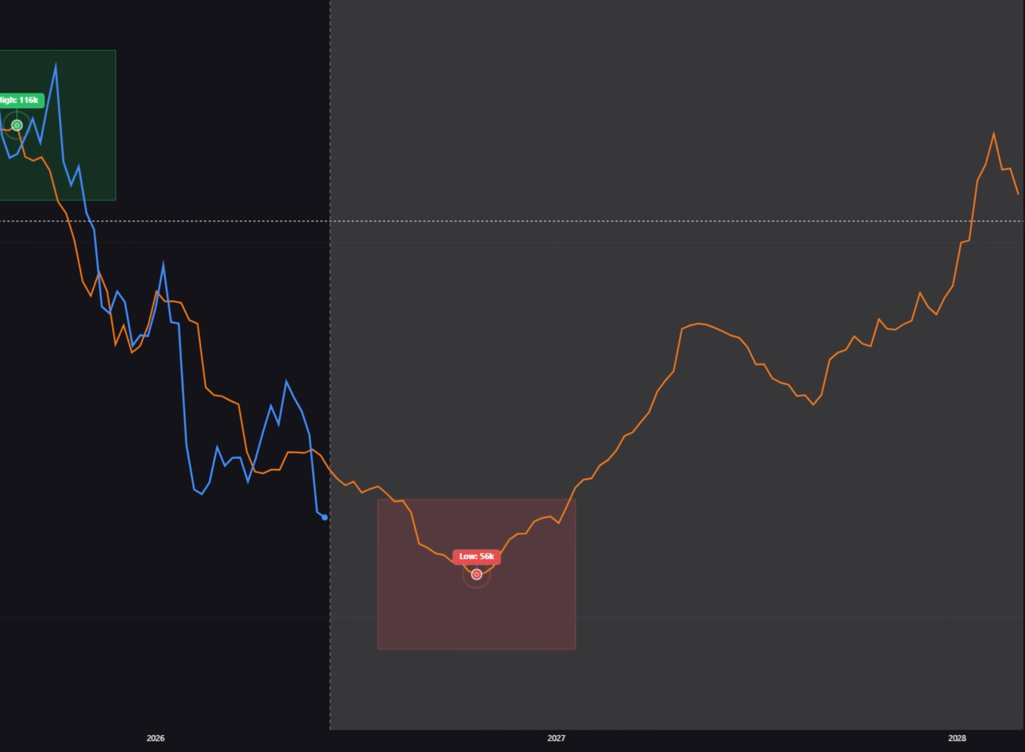
Blue = realized price, orange = model projection. The model has the cycle high at ~$116K, and — critically — does not treat the current drawdown as the bottom. It projects a deeper, more prolonged low around $56K, forming gradually into early 2027, before a sustained recovery back toward new highs in 2028.
This is a completely different methodology — a supervised ML forecast trained on historical price patterns, not the on-chain/cycle-timing overlays above. The fact that it independently lands on a similar multi-quarter bottoming window, rather than confirming the current lows as the floor, is a useful cross-check rather than proof — model forecasts extrapolate from the past and can all be wrong in the same direction if the underlying regime has shifted. It also disagrees with a “the bottom is close” reading in one important way: it projects meaningfully lower prices and a longer grind before recovery, not an imminent V-shaped turn — consistent with the DEFENSIVE signal from the strategy class above. Two independently-built systems, one on-chain/rules-based and one ML-based, both say “not yet, and possibly lower first.”
Where That Leaves the Decision
The calendar-based cycle model: defensive. The trend-following risk overlay: defensive. The value-based overlay (Mayer computed directly, MVRV-Z and Fear/Greed sourced externally): constructive. Two of three model components say “not yet.”
What tips it isn’t any single number — it’s that Mayer Multiple below 1.0 combined with extreme fear has, across the two real historical analogs above, sat closer to the accumulation window than the euphoria window, even though the outcome each time depended on a second-leg-down that isn’t knowable in advance. Given that uncertainty, lump-sum is the wrong instrument; DCA is the one built for “probably right on direction, genuinely unsure on timing.”
So: I’m starting a weekly DCA position. Fixed base amount, no discretionary overrides based on headlines or how a given day feels, sized so that being early costs time rather than solvency. I’m not scaling it up with a value-multiplier — the model’s own two computed components are still defensive, and overriding a model’s output on the strength of two externally-sourced numbers is exactly the kind of talking-myself-into-it this framework exists to avoid.
Key Takeaways
The bear market arrived faster than Part 1’s base case — already in the $50K-70K zone months ahead of the “Q4 2026” estimate.
Re-running Part 1’s own strategy class gives DEFENSIVE, not ACCUMULATE — both the calendar overlay and the trend-following risk overlay are still cautious. The DCA position is additive, not an override.
Mayer Multiple at 0.84 and falling below 1.0 has historically been closer to an accumulation zone than a top— Pi Cycle confirms no top signal is anywhere close.
The DCA-vs-lump-sum backtest is genuinely mixed (+85.2% vs +58.8% in 2018; +28.9% vs +35.5% in 2022)— the honest conclusion is that DCA removes tail risk, not that it reliably outperforms.
An independently-built ML forecasting model projects a deeper, later bottom (~$56K, forming into early-2027) rather than confirming the current lows as the floor — a different methodology landing in a similar multi-quarter window as the on-chain overlay, without either one predicting an imminent turn.
MVRV-Z and Fear/Greed inputs are sourced externally, not computed here — worth knowing which parts of this analysis are independently reproducible and which rest on a tracker.
Conclusion
Part 1 built a framework and let the data say what it would say, including a forecast that turned out a touch conservative on timing. Part 2 points that same framework at itself: when the calendar-based model and the on-chain value model disagree, that disagreement is worth trading systematically rather than picking whichever one currently agrees with what you want to do.
I’m starting to DCA into Bitcoin here — not because the bottom is confirmed, but because the composite evidence has shifted further toward accumulation than at any point since the October 2025 peak, and a rules-based, gradually-scaling DCA is the position sizing that’s honest about how much of that shift is real signal versus how much is still noise.
Happy Trading!
Alex
One more thing. It’s been a couple of months since I personally posted here — studies took over completely for a while and something had to give, and this was it. Good thing Quant Journey is a team effort: Jakub kept things running with regular posts while I was heads-down.
I’m back now, and back properly. There’s a backlog of analysis I’ve wanted to write up, and a lot more of this coming from me — more cycle updates, more strategy breakdowns, more code you can actually run yourself. Thanks for sticking around in the meantime.
Disclaimer: This analysis reflects my own research and personal position-sizing framework, not financial advice. MVRV-Z and Fear & Greed figures are sourced from public trackers as of early July 2026 and should be refreshed before acting on any of this. Cryptocurrency investments carry significant risk. Always conduct your own research and consult with qualified financial advisors before making investment decisions.
 |
|