

In this post, you will read about:
How we generate different Alpha(s) to assess strategy performance
Examples of Alphas that achieved Sharpe Ratios (SR) of 1.92, 1.8, 1.58, etc.
The evaluation of Alphas for both technical and fundamental parameters before feeding them into the backtesting engine
Introduction
An alpha is a combination of mathematical expressions, computer source code, and configuration parameters used with historical data to predict future movements of various financial instruments. Alpha refers to any reasonable expected return that a trader might seek to capitalize on. Alpha represents additional return over a naive forecast.
Often, detailed information about how alphas are constructed may not be available. For instance, the only data available might be the position data, making alpha a set of instructions to achieve certain stock (or other instrument) holdings by specific times.
Many alpha signals can be classified as mean-reversion or momentum-based, but there are also other types such as market making, arbitrage, model-based, and carry, which exploit different market inefficiencies or pricing models.
A mean-reversion alpha's sign opposes its base return. For example, a basic mean-reversion alpha is defined as follows:
−ln(today's open / yesterday's close)
In this scenario, the expectation is that the stock will revert to its mean. If today's opening price is higher than yesterday's close, it might give back some of its gains. Conversely, if today's open is lower than yesterday's close, it might recoup some of the losses.
Another key factor is the timing of the alpha trade. The above alpha would ideally be traded at or, more realistically, as close as possible to today’s open, hence it's called a delay-0 alpha. The terminology used is:
Delay - Data delay
Delay = 1 alphas trade in the morning using data from yesterday
Delay = 0 alphas trade in the evening using data from today
Another example of a momentum alpha is given by:
ln(yesterday′s close / yesterday's open)
The concept here is that if a stock trended yesterday, it would continue today, enhancing gains or losses. This is a delay-1 alpha for immediate trading to maintain the momentum, best starting at the open of the next day.
Generally, delay-0 alphas perform better but have stricter submission requirements. Similarly, delay-2 alphas count the number of days the data used is out-of-sample.
For example:
Alpha #101 - formulated as "((close - open) / ((high - low) + .001))" is a delay-1 momentum alpha: if the stock rises intraday (i.e., close > open and high > low), the next day, one takes a long position in the stock.
Alpha #42 - formulated as "(rank((vwap - close)) / rank((vwap + close)))" is a delay-0 mean-reversion alpha: rank(vwap – close) is lower if a stock rises in the second half of the day (close > vwap) as opposed to falling (close < vwap).
In complex alphas, elements of mean-reversion and momentum can be mixed, making them less distinct.
Building Successful Alphas
Building alpha involves:
Defining your universe with liquidity and other criteria.
Creating raw alpha signals using selected factors and models.
Applying decay to emphasize recent data.
Capping weights to limit stock concentration (in portfolio)
Neutralizing portfolio to desired factors.
Periodically rebalancing portfolio.
Key concepts:
Universe refers to the stocks to which the alpha signal is applied, often filtered based on liquidity to ensure ease of trading without significantly impacting prices.
Decay ensures that alpha signals, reliant on historical data, lose predictive value over time. With linear decay, recent data gains importance over older, smoothing the signal for potentially improved future accuracy.
Weight capping sets a maximum daily weight for each stock in the portfolio to prevent overconcentration in any single stock, thereby reducing idiosyncratic risk and enhancing diversification.
Factor neutralization manages risk exposures and isolates the alpha signal in a portfolio by constructing a portfolio with zero net exposure to certain risk factors such as market beta, sector exposures, or style factors (e.g., value, growth, momentum).
Successful Alphas from WorldQuant
Let's review some successful alphas that WorldQuant has previously published. The status of those alpha is unknown, but you may use them as basic for your alphas’ discovery and successful strategies formulation.
Please note the truncation method here is like weight capping, as mentioned earlier.
USA, TOP3000, Decay 3, Delay 1, Truncation 0.05, Neutralization None
Sharpe 1.39, Turnover 17.15%, Fitness 1.11, Returns 10.87%, Drawdown 8.14%, Margin 12.67%
lookback = 10;
avg_ret = power(ts_product(returns+1, lookback), 1/lookback);
comp_avg = power(ts_product(rel_ret_comp+1, lookback), 1/lookback);
a = zscore(comp_avg / avg_ret);
when = ts_rank(ts_std_dev(returns, 60), 126) > 0.55;
b = trade_when(when, a, -1);
group_vector_neut(b, ts_mean(returns, 120), subindustry)
USA, TOP3000, Decay 5, Delay 1, Truncation 0.1, Neutralization Subindustry
Sharpe 1.94, Turnover 44.52%, Fitness 1.35, Returns 21.66%, Drawdown 11.37%, Margin 9.73%
buzz = ts_backfill(-vec_sum(scl12_alltype_buzzvec), 20);
ts_av_diff(buzz, 60)
CHN, TOP3000, Decay 3, Delay 0, Truncation 0.005, Neutralization Market
Sharpe 5.03, Turnover 13.02%, Fitness 7.52, Returns 29.08%, Drawdown 7.09%, Margin 44.68%
gp = subindustry;
a = rank(-mdl175_volatility * log(volume)) * (1 + group_rank(mdl175_revenuettm,gp));
vector_neut(a, ts_mean(mdl175_02amvt, 240))
group_vector_neut(a, ts_mean(mdl175_02amvt, 50), gp)
USA, TOP3000, Decay 5, Delay 1, Truncation 0.01, Neutralization Subindustry
Sharpe 1.55, Turnover 3.71%, Fitness 1.18, Returns 7.28%, Drawdown 7.11%, Margin 39.28%
-ts_rank(retained_earnings,500)
USA, TOP200, Decay 10, Delay 1, Truncation 0.01, Neutralization Subindustry
Sharpe 1.62, Turnover 2.21%, Fitness 1.52, Returns 11.06%, Drawdown 11.65%, Margin 100.21%
-rank(ebit/capex)
USA, TOP1000, Decay 10, Delay 1, Truncation 0.01, Neutralization Market
Sharpe 1.38, Turnover 2.00%, Fitness 1.35, Returns 12.04%, Drawdown 13.20%, Margin 120.20%
group_rank(fam_est_eps_rank, sector)
USA, TOP3000, Decay 1, Delay 1, Truncation 0.05, Neutralization Market
Sharpe 1.59, Turnover 2.79%, Fitness 1.70, Returns 14.33%, Drawdown 7.53%, Margin 102.66%
a = ts_av_diff(mdf_eg3, 50);
b = ts_corr(mdf_eg3, mdf_sg3, 50);
-a * b
USA, TOP500, Decay 1, Delay 1, Truncation 0.01, Neutralization Subindustry
Sharpe 1.28, Turnover 1.91%, Fitness 1.15, Returns 10.17%, Drawdown 8.18%, Margin 106.23%
rank(mdf_rds)
USA, TOP3000, Decay 30, Delay 1, Truncation 0.01, Neutralization Subindustry
Sharpe 1.84, Turnover 8.99%, Fitness 1.08, Returns 4.29%, Drawdown 1.93%, Margin 9.55%
avg_news = vec_avg(nws12_afterhsz_sl);
rank(ts_sum(avg_news, 60)) > 0.5 ? 1 : rank(-ts_delta(close, 2))
USA, TOP3000, Decay 0, Delay 1, Truncation 0.1, Neutralization Subindustry
Sharpe 1.79, Turnover 14.71%, Fitness 1.24, Returns 7.10%, Drawdown 6.82%, Margin 9.65%
ts_zscore(mdf_oey, 250)
USA, TOP200, Decay 10, Delay 1, Truncation 0.05, Neutralization Market
Sharpe 1.58, Turnover 49.64%, Fitness 1.09, Returns 23.76%, Drawdown 10.30%, Margin 9.57%
decay_days = 1;
rel_days_since_max = rank(ts_arg_max(close, 30));
decline_pct = (vwap - close) / close;
decline_pct / min( ts_decay_linear(rel_days_since_max, decay_days), 0.15)
USA, TOP3000, Decay 10, Delay 1, Truncation 0.01, Neutralization Subindustry
Sharpe 1.92, Turnover 48.92%, Fitness 0.99, Returns 13.01%, Drawdown 8.25%, Margin 5.32%
decay_days = 2;
rel_days_since_max = rank(ts_arg_max(close, 30));
decline_pct = (vwap - close) / close;
decline_pct / min( ts_decay_linear(rel_days_since_max, decay_days), 0.20)
Upon observation, you will notice that most of these alphas are simple in their structure. They seldom extend beyond 5-6 factors. This simplicity is a noteworthy characteristic, indicating a certain degree of restraint in their design while still effectively fulfilling their purpose.
Let's begin coding our assessment of the alpha.
The previously written module, alpha_expression.py, accepts the Formulaic Alpha in the following form:
"1": "(rank(ts_argmax(signedpower(((returns < 0) ? stddev(returns, 20) : close), 2.), 5)) - 0.5)",
And converts it into a more Python-aware form:
expressions = {
		"1": "(rank(ts_argmax(signedpower((stddev(returns, 20) if (returns < 0) else close), 2.), 5)) - 0.5)",
	}
Our goal is to calculate the value of the expression (alpha) for different equities on each day within the analysis period.
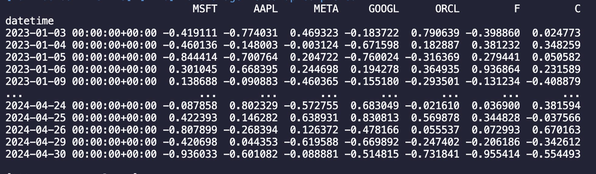
To achieve this, we begin by parsing the alpha expression. Next, we evaluate each factor and apply the required operations to the retrieved data for each equity.
We will use the Abstract Syntax Tree library for this purpose and formulate an AlphaEval class:
class AlphaEval:
	def __init__(self, verbose = None):
		self.eval_functions = EvalFunctions()
		self.verbose = verbose

	def evaluate_expression(self, expression, data):
		"""
		Evaluate the given expression using the provided data.
		"""
		try:
			nodes = ast.parse(expression, mode='eval')							# Generate AST (Abstract Syntax Tree)
			result, _ = self.evaluate_node(nodes.body, data, [])				# Evaluate the AST
			return result
		except SyntaxError as e:
			logger.error(f"Syntax error in expression: {expression}, Error: {e}")
			return None
The function ast.parse(expression) generates a tree of 'child nodes', e.g.:
('(returns < 0)'
('stddev(returns, 20)')
('((returns < 0) ? stddev(returns, 20) : close)', 0)
('ts_argmax(signedpower(((returns < 0) ? stddev(returns, 20) : close), 2.0), 5)', 0)
 ('rank(ts_argmax(signedpower(((returns < 0) ? stddev(returns, 20) : close), 2.0), 5))', 0)
All nodes are processed by the evaluate_node function. This function traverses each node, deriving values from functions like signedpower, stddev, ts_argmax, and rank. These functions are accessible via the EvalFunctions class, which houses over 60 similar functions designed to evaluate any alpha expression.
def evaluate_node(self, node, data, steps):
		"""
		Evaluate the AST recursively.
		"""
		if isinstance(node, ast.BinOp):  										# Binary operator (arithmetic and bitwise operations)
			left, steps = self.evaluate_node(node.left, data, steps)
			right, steps = self.evaluate_node(node.right, data, steps)
			result = self._apply_binop(node.op, left, right)
			steps.append((self.node_to_str(node), result))
			return result, steps

		elif isinstance(node, ast.UnaryOp):  									# Unary operator (operations like positive, negative, logical NOT, and bitwise NOT)
			operand, steps = self.evaluate_node(node.operand, data, steps)
			result = self._apply_unaryop(node.op, operand)
			steps.append((self.node_to_str(node), result))
			return result, steps

		elif isinstance(node, ast.Constant):  									# Constant values (numbers, strings, etc.)
			return node.value, steps

		elif isinstance(node, ast.Name):  										# Handling variables like open, close, high, low, volume
			if node.id not in data:
				try:
					data[node.id] = getattr(self.eval_functions, node.id)(pd.DataFrame(data))  # From EvalFunctions trying other functions e.g. vwap, adv, etc.
				except AttributeError:
					raise KeyError(f"'{node.id}' not found in data and no corresponding function found in EvalFunctions.")
			return data[node.id], steps

		elif isinstance(node, ast.Call):  										# Handling function calls
			if isinstance(node.func, ast.Name):
				func = getattr(self.eval_functions, node.func.id)				# From EvalFunctions trying other functions e.g. vwap, adv, etc.
			elif isinstance(node.func, ast.Attribute):
				module = getattr(self.eval_functions, node.func.value.id)
				func = getattr(module, node.func.attr)
			else:
				raise ValueError(f"Unsupported function type: {type(node.func)}")

			args = [self.evaluate_node(arg, data, steps)[0] for arg in node.args]
			result = func(*args)
			steps.append((self.node_to_str(node), result))
			return result, steps

		elif isinstance(node, ast.Compare):  									# Comparison operations (==, !=, <, <=, >, >=, is, is not, in, not in)
			left, steps = self.evaluate_node(node.left, data, steps)
			right, steps = self.evaluate_node(node.comparators[0], data, steps)
			result = self._apply_compare(node.ops[0], left, right)
			steps.append((self.node_to_str(node), result))
			return result, steps

		elif isinstance(node, ast.IfExp):  										# Conditional expressions (ternary operator)
			test, steps = self.evaluate_node(node.test, data, steps)
			body, steps = self.evaluate_node(node.body, data, steps)
			orelse, steps = self.evaluate_node(node.orelse, data, steps)
			result = pd.Series(np.where(test, body, orelse))
			steps.append((self.node_to_str(node), result))
			return result, steps

		elif isinstance(node, ast.Attribute):  									# Attribute access (e.g. close, open, high, low, volume)
			value, steps = self.evaluate_node(node.value, data, steps)
			result = getattr(value, node.attr)
			steps.append((self.node_to_str(node), result))
			return result, steps

		else:
			raise ValueError(f"Unsupported AST node: {node}")
As you can see, there are different conditions and operators, including binary and unary operators, as well as comparators.
Once that is complete, we can apply other rules such as delay and decay to generate signals. A simple function to do this could look like this:
def generate_signals(df, buy_threshold=0.3, sell_threshold=0.2):
	signals = pd.DataFrame(index=df.index, columns=df.columns)
	for ticker in df.columns:
		signals[ticker] = np.where(df[ticker] > buy_threshold, 'Buy',
								   np.where(df[ticker] < sell_threshold, 'Sell', 'Hold'))
	return signals
providing results such as:

I'm working on a more complex version of generate_signals function in the QuantJourney framework, which will be used to maximize outcomes from each strategy. It’s more related to signal events and will be published in the next few weeks.
Additional Potential Alphas
If you're reach this part, please note that we can blend alpha expressions not only with simple elements but also with technical and even fundamental ones.
Alpha Expression 105: VWAP, Volume, and Return on Equity (ROE)
"105": "(rank(correlation(TI.vwap(data), data['Volume'], 4.24)) < rank(correlation(rank(data['Low']), rank(FI.return_on_equity(data, year=2023)), 12.44)))"
This signal compares the correlation of VWAP with volume against the correlation of low prices with return on equity. It can identify opportunities where price action related to volume is less influential than fundamental performance, suggesting potential undervaluation.
Alpha Expression 106: Power, Rank, and Correlation with Net Profit Margin:
"106": "np.power(rank(correlation(TI.ts_sum(((data['Low'] * 0.35) + (TI.vwap(data) * 0.65)), 20), TI.ts_sum(FI.net_profit_margin(data, year=2023), 20), 7)), rank(correlation(rank(TI.vwap(data)), rank(data['Volume']), 6)))"
This signal evaluates the correlation of weighted price sums with net profit margins and compares it to VWAP-volume correlation. It aims to find instances where both technical movements and fundamental profitability are aligned.
Alpha Expression: 134: Log Product of Rank and Power with Price-to-Earnings Ratio
"134": "((rank(np.log(np.product(rank(np.power(rank(correlation(TI.vwap(data), TI.ts_sum(FI.price_to_earnings(data, year=2023), 50), 8)), 4)), 15))) < rank(correlation(rank(TI.vwap(data)), rank(data['Volume']), 5))) * -1)"
This signal uses the log product of ranked correlations with the price-to-earnings ratio. It is useful for identifying when price movements strongly correlate with earnings, potentially signaling overbought or oversold conditions.
Extending AST with Technical and Fundamental formulas
For such alphas we must extend our AlphaEval class to understand three categories of elements in alpha’s expression:
General entries, which include open, close, high, low, volume as well as functions like ABS, NEG, TS_ARG_MAX, RANK, and so on.
Technical entries, such as SMA, EMA, VWAP, OBV, along with more complex indicators like ATR, ADX, WILLR, and so on.
Fundamental entries, including EBIT, CAPEX, ROA, ROE, Current Ratio, MCAP, PE, FCF, PEG, and others.
Here, we construct three supportive classes. Adopting a modular approach keeps things straightforward and minimizes potential issues.
First, the EvalFunctions class, which covers 62 key methods:
class EvalFunctions:

    @staticmethod
    def signedpower(series, power):
        return np.sign(series) * (abs(series) ** power)

    @staticmethod
    def sum(series, window):
        return series.rolling(window).sum()

    @staticmethod
    def ts_sum(series, window=10):
        return series.rolling(window).sum()

    @staticmethod
    def sma(series, window=10):
        return series.rolling(window).mean()

    @staticmethod
    def stddev(series, window=10):
        return series.rolling(window).std()

    @staticmethod
    def correlation(series_a, series_b, window=10):
        return series_a.rolling(window).corr(series_b)
Secondly, there's EvalTechnical. This is based on the already written technical_indicators.py module from the QuantJourney Framework, which includes over 100 different technical indicators.
class EvalTechnical:

	@staticmethod
	def rsi_series(series, window):
		return TI.RSI(series, window=window)

	@staticmethod
	def sma_series(series, window):
		return TI.SMA(series, window=window)

	@staticmethod
	def ema_series(series, window):
		return TI.EMA(series, window=window)

	@staticmethod
	def bb_series(series, window, nb_std_dev=2):
		return TI.BB(series, window=window, nb_std_dev=nb_std_dev)

	@staticmethod
	def atr_series(series, window):
		return TI.ATR(series, window=window)
Third, we have 'EvalFundamental'. This is based on the previously written 'fundamental_indicators.py' module which fetches fundamental data for each equity. It calculates key ratios directly from Profit & Loss data, including balance sheet, cash flow, and income statement data.
async def net_profit_margin(self, ticker: str, exchange: str, source: str, year: int, quarter: Union[int, None] = None, specific_date: Optional[str] = None):
		"""
		Calculate the net profit margin
  		"""
		try:
			period = 'q' if quarter or specific_date else 'y'

			income_statement_data = await self._get_cached_fundamental_data(ticker, exchange, source, 'income_statement', period, specific_date)
			if income_statement_data.empty:
				logger.error(f"No data available for {ticker} in {exchange} from {source}.")
				return None

			income_statement_filtered = self.filter_data(income_statement_data, year, quarter, specific_date)
			if isinstance(income_statement_filtered, pd.Series):
				income_statement_filtered = pd.DataFrame(income_statement_filtered).T

			income_statement_filtered['netIncome'] = pd.to_numeric(income_statement_filtered['netIncome'], errors='coerce')
			income_statement_filtered['totalRevenue'] = pd.to_numeric(income_statement_filtered['totalRevenue'], errors='coerce')

			income_statement_filtered['net_profit_margin'] = income_statement_filtered['netIncome'] / income_statement_filtered['totalRevenue']
			income_statement_filtered['net_profit_margin'].replace([np.inf, -np.inf, np.nan], 0, inplace=True)

			logger.info(f"Net profit margin calculated successfully for {ticker}.")
			return income_statement_filtered['net_profit_margin']

		except Exception as e:
			logger.error(f"Failed to calculate net profit margin for {ticker}: {e}")
			return None
And the class appears as follows in EvalFundamental:
class EvalFundamental:

	@staticmethod
	def gross_profit_margin(series, **kwargs):
		return FI.gross_profit_margin(series, **kwargs)

	@staticmethod
	def operating_profit_margin(series, **kwargs):
		return FI.operating_profit_margin(series, **kwargs)

	@staticmethod
	def net_profit_margin(series, **kwargs):
		return FI.net_profit_margin(series, **kwargs)

	@staticmethod
	def return_on_assets(series, **kwargs):
		return FI.return_on_assets(series, **kwargs)

	@staticmethod
	def return_on_equity(series, **kwargs):
		return FI.return_on_equity(series, **kwargs)

	@staticmethod
	def debt_to_equity(series, **kwargs):
		return FI.debt_to_equity(series, **kwargs)

	@staticmethod
	def current_ratio(series, **kwargs):
		return FI.current_ratio(series, **kwargs)

	@staticmethod
	def quick_ratio(series, **kwargs):
		return FI.quick_ratio(series, **kwargs)

	@staticmethod
	def cash_flow_to_debt(series, **kwargs):
		return FI.cash_flow_to_debt(series, **kwargs)
By utilizing these classes, we can generate Alpha expressions like WorldQuant in a single line. This is aligned with the purpose of the QuantJourney Framework, to demonstrate the robustness of our system and the efficiency of our methods.
Conclusion
In conclusion, we will present the results of the alpha used ("1": "(rank(ts_argmax(signedpower(((returns < 0) ? stddev(returns, 20) : close), 2.), 5)) - 0.5)"). The signals were run through our backtesting engine for the equities MSFT and META, from January 2023 to the present. The plot depicts the cumulative returns for each equity according to this alpha.

Although this is before additional parameterization and optimization, the progression from a basic alpha expression to its evaluation is straightforward. It can then be enhanced with technical and fundamental factors to generate results.