Hierarchical Portfolio Construction: A Smarter Approach to Asset Allocation

In This Post, You Will Read About:

• Why Traditional Portfolio Optimization Falls Short → The limitations of mean-variance optimization and why correlation estimates are often unreliable.

• How Hierarchical Portfolio Construction (HPC) Works → Using clustering to create a more stable and intuitive diversification framework.

• Implementing HPC in QuantJourney → Applying the HierarchicalPortfolioOptimizer inside the QuantJourney backtester for real-world portfolio allocation.

Why Move Beyond Traditional Portfolio Optimization?

Traditional portfolio optimization (like Markowitz's mean-variance approach) treats all assets as one big pool. While this might sound reasonable, it often leads to unstable portfolios that don't perform well in the real world. Why? Because estimating correlations and covariance matrices across many assets is difficult and error-prone.

One well-known improvement is the Black-Litterman model, which blends investor views with historical data for more stable allocations. While this helps, it still relies on estimating correlations, which can be unreliable - especially with many assets.

That’s where hierarchical methods step in.

Instead of trying to understand how every asset relates to every other asset at once, hierarchical approaches first cluster similar assets, then allocate capital across these clusters. This approach is:

1. More Natural – Stocks in the same sector (e.g., Tech) usually move together.

2. More Stable – Group-level relationships are often more reliable than individual pairwise correlations.

3. More Flexible – You can adapt the grouping logic (linkage methods, distance metrics, etc.) to your own needs or views.

QuantJourney's Portfolio Optimization Framework

Within the QuantJourney framework, multiple portfolio construction techniques are already implemented, allowing for flexibility in choosing the best optimization model for a given strategy:

quantjourney/portfolio/optimizers
├── base_optimizer.py
├── black_litterman_optimizer.py
├── mean_variance_optimizer.py
├── optimizer_calculations.py
├── optimizer_registry.py
├── portfolio_optimizer.py
├── risk_parity_optimizer.py

Hierarchical Portfolio Construction (HPC) is a broader approach that groups assets before optimizing portfolio weights. This method can be used with Black-Litterman, Mean-Variance, and Risk Parity models to improve stability and reduce sensitivity to noisy correlations.

One well-known variation is Hierarchical Risk Parity (HRP), developed by López de Prado. HRP applies risk parity principles within a hierarchical structure, offering an alternative to traditional covariance-based optimizations.

By leveraging QuantJourney’s structure, users can combine hierarchical clustering with traditional optimization techniques, achieving a more stable and flexible portfolio allocation.

A Bird’s-Eye View of Hierarchical Portfolio Construction

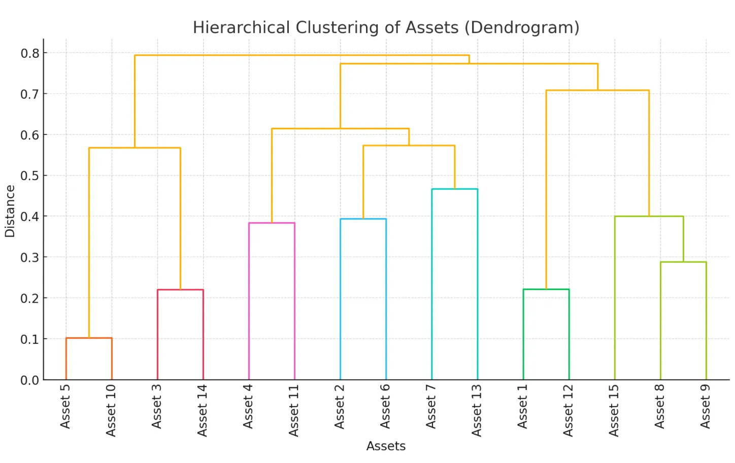
Hierarchical Portfolio Construction (HPC) organizes assets (or whole asset classes) into a multi-level structure - like a family tree of investments. This structure (called a dendrogram) helps visualize how assets relate in terms of risk, correlation, and return potential.

1. Top-Down (Root Node) → The entire portfolio sits at the root, representing broad diversification (e.g., stocks vs. bonds).

2. Intermediate Clusters → Each branch groups assets based on correlation (e.g., “Large-Cap Tech” vs. “Mid-Cap Healthcare”).

3. Leaves (Individual Stocks) → At the bottom, individual assets are assigned precise portfolio weights.

Here’s an example dendrogram, illustrating hierarchical asset grouping:

Computational Framework

A key principle in hierarchical portfolio construction is separating structure from allocation methodology. The process consists of two stages:

1. Dendrogram Construction – Clustering assets into a hierarchical tree using statistical distance measures (e.g., Ward’s method, single linkage).

2. Weight Calculation – Applying portfolio allocation models on top of this structure. Common allocation methods include:

   • Traditional Mean-Variance Optimization

   • Equal Weighting (1/n)

   • Risk Parity Approaches (including HRP)

Implementation Example

Consider a universe of 20 US stocks. A hierarchical clustering process might reveal three major asset clusters, with further subdivisions. If an equal-weighted (1/n) strategy is applied to these clusters, each receives 33% of the portfolio’s capital. However, this could lead to counterintuitive allocations - for example, a smaller stock like Best Buy might receive a higher weight than Amazon, depending on the clustering structure.

A dendrogram visualization helps to understand these relationships and refine weight allocation strategies.

Practical Considerations

How often should you update clusters? Too frequent updates lead to excessive rebalancing (higher costs), while too infrequent updates might miss changes in market structure. A common approach is to adjust clusters monthly or quarterly, depending on market conditions. The top-level split (root node) is crucial, as it influences all subsequent capital allocations.

The Bisection Debate

López de Prado's Hierarchical Risk Parity (HRP) method introduces an additional bisection step, which involves:

• Constructing an initial dendrogram.

• Extracting the asset order.

• Creating a new dendrogram that forces equal-sized top-level clusters.

This technique sometimes disrupts natural clusters. For instance, in a portfolio of 11 stocks and 9 bonds, an automated bisection process might mix asset classes rather than keeping them in separate clusters, which contradicts fundamental investment principles.

Why Does Hierarchical Portfolio Construction Matter?

• Natural Clustering: Markets are hierarchical by nature (think about how you’d categorize stocks by sector, region, or style).

• Risk Segmentation: HPC makes it easy to allocate risk across top-level clusters and refine allocations within them.

• Robustness: Research from Thomas Raffinot and Marcos López de Prado shows that hierarchical methods often outperform classical mean-variance optimization, reducing sensitivity to covariance estimation errors.

How Does It Work? A Simple Example

Let’s take a 15-stock portfolio across three major sectors:

• Tech: AAPL, MSFT, GOOGL, AMZN, NVDA

• Healthcare: JNJ, PFE, MRK, ABBV, UNH

• Finance: JPM, BAC, WFC, C, GS

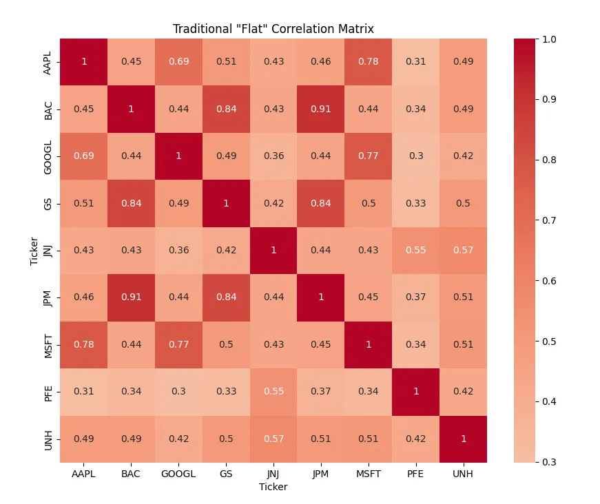
Instead of estimating the full covariance matrix (flat), hierarchical methods:

1. Group assets within each sector using hierarchical clustering.

2. Allocate Capital Across Sectors → (e.g., 40% Tech, 30% Healthcare, 30% Finance).

3. Sub-Allocate within each sector (e.g., within Tech, giving more weight to lower-volatility stocks).

This avoids overfitting to correlation noise and results in more diversified portfolios.

See below:

Implementing Hierarchical Portfolios with QuantJourney

In QuantJourney, we use a hierarchical optimizer that performs:

• Cluster Building: Using hierarchical clustering (e.g., Ward’s method) to create a dendrogram.

• Bisection: Optionally splitting large clusters into more balanced ones (a common technique of López de Prado).

• Traversal: Whether to allocate top-down (vertical recursion) or via a simpler, one-level (horizontal) approach.

• Integration with a Backtester: Periodically recalculate the hierarchical clusters, then update your portfolio weights accordingly.

1) Strategy Configuration

In QuantJourney, you’ll typically define a strategy configuration that includes your universe of instruments, initial capital, and rebalancing rules:

strategy_config = {
    "strategy_name": "HierarchicalPortfolio",
    "initial_capital": 100000,
    "instruments": [
        "AAPL", "MSFT", "GOOGL", "AMZN", "NVDA",  # Tech
        "JNJ", "PFE", "MRK", "ABBV", "UNH",       # Healthcare
        "JPM", "BAC", "WFC", "C", "GS"            # Finance
    ],
    "trading_range": {
        "start": "2020-01-01",
        "end": "2024-12-31"
    },
    "risk_management": {
        "global": {
            "max_position_weight": 0.2,
            "target_volatility": 0.15
        }
    }
}

2) Building a Hierarchical Optimizer

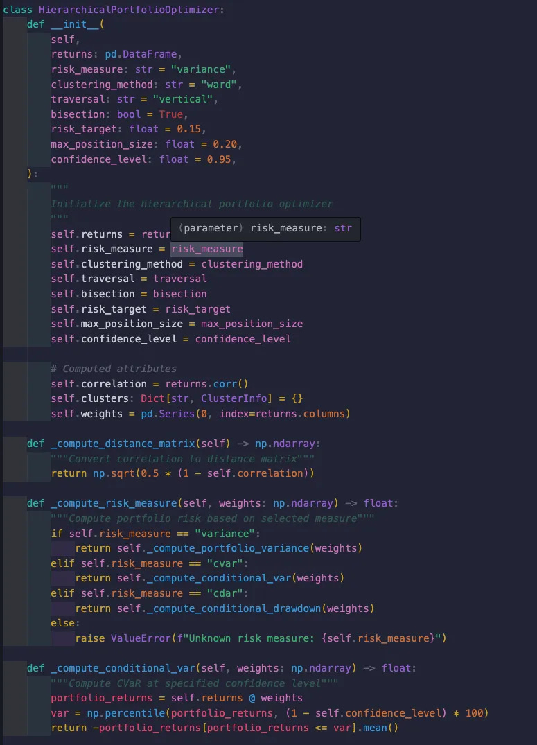
Let’s assume you have a custom optimizer in quantjourney.portfolio.optimisation that handles hierarchical clustering, risk measures, and bisection:

This implementation includes:

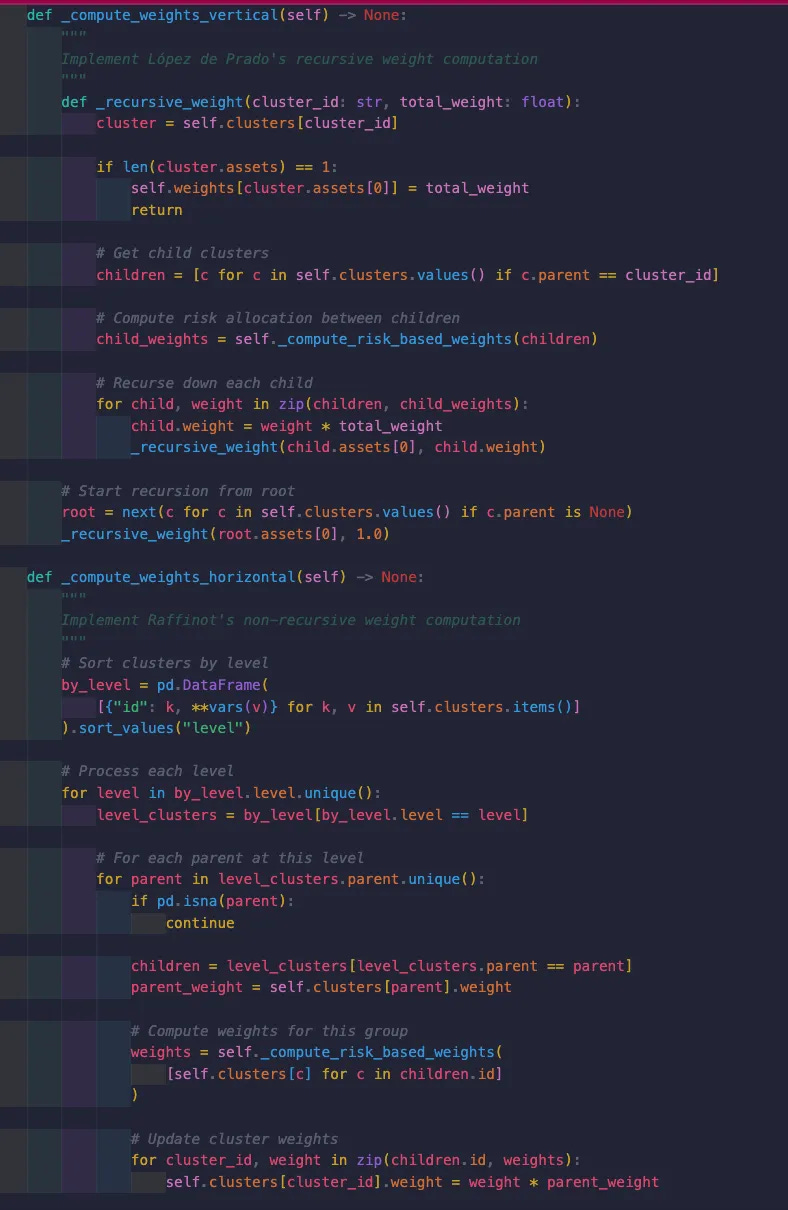
1. Both vertical (López de Prado) and horizontal (Raffinot) traversal methods

2. Advanced risk measures (variance, CVaR, CDaR)

3. Proper error handling and validation

4. Visualization capabilities

5. Performance scaling to hit risk targets

and:

How to use it:

from quantjourney.portfolio.optimizers import HierarchicalPortfolioOptimizer

self.optimizer = HierarchicalPortfolioOptimizer(
    returns=self.instruments_data.get_returns(window=self.lookback_period),
    risk_measure="cdar",  # Conditional Drawdown at Risk
    clustering_method="ward",
    traversal="vertical",  # Lopez de Prado's recursive method
    bisection=True,  # Balanced clusters
)

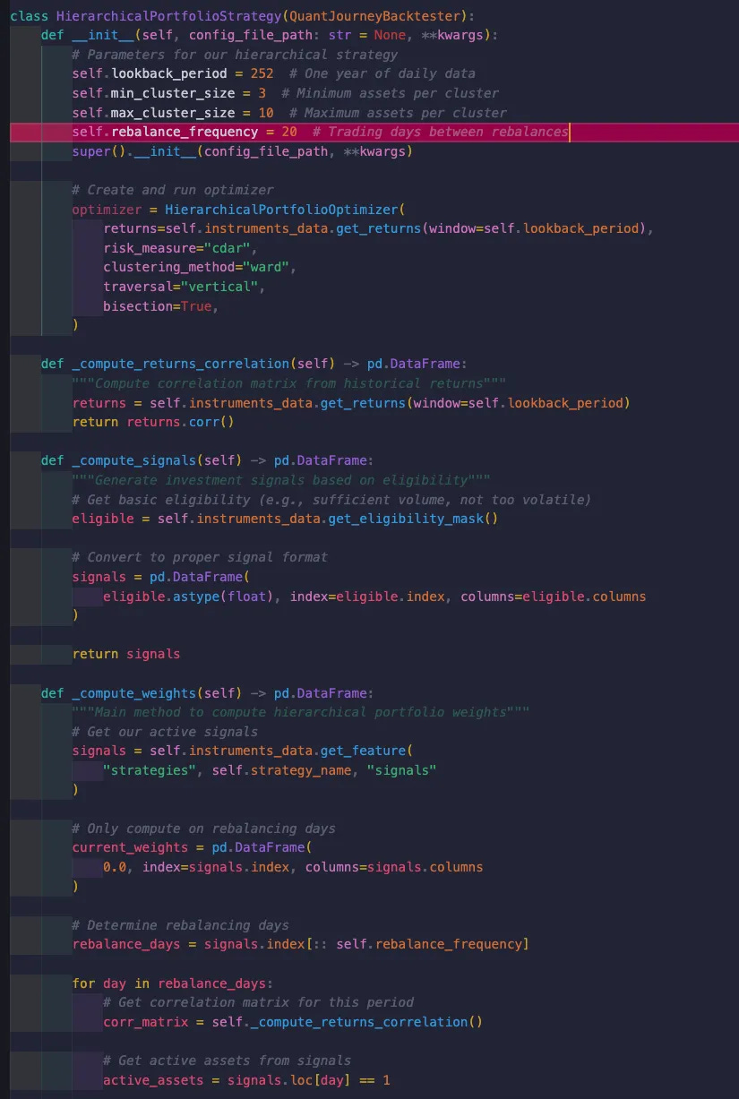
3. A Hierarchical Strategy for the QuantJourney Backtester

We then define a backtester-based strategy that calculates signals (if any) and uses our hierarchical optimizer for weights:

4) Running the Strategy

You can now instantiate and run your strategy just as with any QuantJourney backtester:

strategy = HierarchicalPortfolioStrategy(**strategy_config)
results = await strategy.run_strategy()

Interpreting the Results

1. Clusters Form: On each rebalance day, the optimizer clusters the active assets. If bisection is enabled, it further splits large clusters for balance.

2. Weights Computed: The vertical (recursive) approach sets allocations at each sub-branch of the tree, ultimately generating an asset-level weight vector.

3. Portfolio Execution: The backtester invests in proportion to these hierarchical weights until the next rebalance day.

4. Performance Monitoring: You can track metrics like Sharpe ratio, drawdown, and turnover to see how the strategy performs vs. a simpler mean-variance or equal-weight approach.

---

Frequently Asked Questions

Q: How often should I rebalance?

A: A monthly or quarterly frequency is common to strike a balance between capturing changes in asset relationships and controlling transaction costs. Adjust based on your strategy’s sensitivity to market regimes.

Q: What’s the best clustering method (Ward’s, single linkage, average linkage)?

A: Ward’s method often works well in finance, but there’s no universal “best.” Experiment with different linkage approaches to see which yields more stable allocations for your universe.

Q: How do I handle discrete shares?

A: The weights generated by hierarchical methods are continuous. If you need to place real trades, you’ll likely need a post-processing step that transforms these weights into integer share quantities - e.g., using a greedy or integer programming approach. (Stay tuned for more on that in upcoming posts.)

Q: Can I incorporate advanced risk measures (like CVaR)?

A: Absolutely - just replace risk_measure="variance" with a method that computes downside risk. The HPC framework remains the same, but the weight‐allocation logic inside _compute_risk_weights() or _apply_constraints() will need to accommodate CVaR/CDaR.

---

In Summary

Hierarchical portfolio construction offers a practical way to build more stable portfolios by grouping similar assets before applying weight allocation. This reduces reliance on noisy correlation estimates and can work alongside traditional models like Black-Litterman or Risk Parity.

By integrating HPC into the QuantJourney BackTester, you can test different clustering methods and allocation strategies to see what works best for your portfolio. If you're looking for a more resilient way to optimize portfolios, HPC is worth exploring.

Happy investing!

Jakub