
Reinforcement Learning for Trading, from Scratch
A from-scratch introduction to reinforcement learning for trading: we build a Q-learning agent in plain numpy, check it works on synthetic data, then run it on real Bybit data.

TL;DR: We build a Q-learning trading agent from scratch and test it first on synthetic mean-reverting data, where it learns a profitable mean-reversion policy, and then on 20,000 real BTC/USDT 15-minute bars. Out of sample, nine of ten agents stay completely flat; the only one that trades loses 5.7%. The main lesson is not that RL fails, but that once transaction costs and real market noise enter the problem, finding no trade can be a perfectly rational outcome. In trading RL, state design, reward design, costs, and honest out-of-sample validation matter far more than making the learning algorithm more sophisticated.
Reinforcement learning is appealing to traders for a simple reason. Supervised learning predicts: “will the price go up?” RL decides: “given what I know right now, what should I do?” And that’s the question you actually face when trading. Prediction and action are not the same thing. A model that’s right 55% of the time can still lose money if it’s wrong at the worst moments. An RL agent optimizes the thing you actually care about, which is cumulative P&L after costs.
That’s the promise. The reality is messier, and we’ll get to that. But the best way to understand any of this is to build the whole pipeline yourself: environment, agent, training loop, out-of-sample evaluation. So that’s what we’ll do.
By the end of this post you’ll have:
A gym-style trading environment you fully understand, because you wrote it
A tabular Q-learning agent, the simplest version of RL and a good way to learn the mechanics
An out-of-sample equity curve on synthetic data, and then the same agent’s results on real BTC/USDT data from Bybit, which turned out to be the most interesting part
Part one runs with just numpy and matplotlib. Copy, paste, run.
The basics, in trading terms
RL has four core concepts.
Agent: your trading strategy. It observes the market and picks an action.
State: what the agent sees before deciding. In our case, how stretched the price is relative to its recent mean (a bucketed z-score), plus the position we currently hold. Keeping the current position in the state matters. Whether to stay long is a different question than whether to go long, because changing your mind costs money.
Action: what the agent can do. We keep it simple: flat, long, or short. One unit, no sizing.
Reward: the feedback signal. Ours is the one-step return of the position held, minus transaction costs whenever the position changes. This is the crucial design decision in trading RL, because the reward defines what “good” means. Reward raw P&L and the agent learns to gamble. Forget costs and it learns to churn. We’ll charge 1 basis point per position change to keep it honest.
The agent’s job is to learn a policy: a rule mapping states to actions that maximizes cumulative reward.
Q-learning in one paragraph
Q-learning maintains a table Q[state][action], which is an estimate of “how much total future reward do I get if I take this action in this state, and act well afterwards?” After every step it nudges its estimate toward reality:
Q(s, a) ← Q(s, a) + α · [ r + γ · max Q(s', ·) − Q(s, a) ]The bracket is the temporal-difference error: the gap between what we predicted and what we just observed (immediate reward r plus the discounted value of the best move from the next state). α is the learning rate, γ the discount factor. During training the agent explores with probability ε, meaning it acts randomly to discover the state space, and exploits otherwise, with ε decaying over time. That’s genuinely all there is to it. Deep RL replaces the table with a neural network, but the logic stays the same.
Step 1: A market to learn on
We’ll start with a synthetic mean-reverting price series (an Ornstein-Uhlenbeck process). Two reasons. First, it’s self-contained: no API keys, no data downloads, the code runs anywhere. Second, and more importantly, we know the ground truth. A mean-reverting market rewards buying dips and selling rips, so we can check whether the agent learned the right lesson instead of staring at an equity curve and guessing.
import numpy as np
import matplotlib.pyplot as plt

rng = np.random.default_rng(42)

def make_prices(n=4000, mu=100.0, theta=0.05, sigma=1.0):
    prices = np.empty(n)
    prices[0] = mu
    for t in range(1, n):
        prices[t] = prices[t-1] + theta * (mu - prices[t-1]) + sigma * rng.standard_normal()
    return prices

prices = make_prices()
train_prices = prices[:3000]
test_prices = prices[3000:]
Note the split. The agent trains on the first 3,000 bars and gets evaluated on the last 1,000, which it never sees during training.
Step 2: The environment
The environment is the game the agent plays. It hands out states, accepts actions, and pays rewards. We follow the classic gym interface (reset() and step(action)), so everything you learn here transfers directly to gymnasium and stable-baselines3 later.
class TradingEnv:
    """
    State  : (z-score bucket of price vs. rolling mean, current position)
    Action : 0 = flat, 1 = long, 2 = short
    Reward : position * price change - transaction costs
    """
    def __init__(self, prices, window=50, cost_bps=1.0):
        self.prices = prices
        self.window = window
        self.cost = cost_bps / 10_000  # bps -> fraction
        self.n_z_buckets = 9
        self.reset()

    def _zscore(self, t):
        w = self.prices[t - self.window:t]
        sd = w.std() + 1e-9
        return (self.prices[t] - w.mean()) / sd

    def _bucket(self, z):
        edges = [-2, -1.5, -1, -0.5, 0.5, 1, 1.5, 2]
        return int(np.digitize(z, edges))  # 0..8

    def state(self):
        return (self._bucket(self._zscore(self.t)), self.position)

    def reset(self):
        self.t = self.window
        self.position = 0  # -1 short, 0 flat, +1 long
        return self.state()

    def step(self, action):
        new_pos = {0: 0, 1: 1, 2: -1}[action]
        price_now = self.prices[self.t]
        price_next = self.prices[self.t + 1]

        pnl = new_pos * (price_next - price_now) / price_now
        trade_cost = abs(new_pos - self.position) * self.cost
        reward = pnl - trade_cost

        self.position = new_pos
        self.t += 1
        done = self.t >= len(self.prices) - 1
        return self.state(), reward, done
A few details worth noting.
The z-score is computed on a window that excludes the future: we only use prices[t-window:t] plus the current price. Look-ahead bias is the easiest way to build a strategy that looks great in a backtest and fails live.
We bucket the z-score into 9 discrete bins because tabular Q-learning needs a finite state space. With 9 buckets times 3 positions we have at most 27 states. Small enough to learn quickly, but enough to capture “stretched vs. fair”.
The reward is taxed on turnover. abs(new_pos - old_pos) is 0 if you hold, 1 if you enter or exit, and 2 if you flip from long to short. Flipping costs double. This small term has a big effect on behavior, as you’ll see.
Step 3: The agent
class QAgent:
    def __init__(self, n_actions=3, alpha=0.1, gamma=0.99,
                 eps=1.0, eps_min=0.05, eps_decay=0.98):
        self.Q = {}
        self.n_actions = n_actions
        self.alpha, self.gamma = alpha, gamma
        self.eps, self.eps_min, self.eps_decay = eps, eps_min, eps_decay

    def q(self, s):
        if s not in self.Q:
            self.Q[s] = np.zeros(self.n_actions)
        return self.Q[s]

    def act(self, s, greedy=False):
        if not greedy and rng.random() < self.eps:
            return rng.integers(self.n_actions)
        return int(np.argmax(self.q(s)))

    def learn(self, s, a, r, s_next, done):
        target = r if done else r + self.gamma * self.q(s_next).max()
        self.q(s)[a] += self.alpha * (target - self.q(s)[a])
That’s the entire agent. act implements ε-greedy exploration, and learn is the Q-learning update from earlier, verbatim. The Q-table is a dictionary that lazily creates entries, which is plenty at this scale.
Step 4: Train, then evaluate on unseen data
def train(agent, env, episodes=200):
    episode_returns = []
    for _ in range(episodes):
        s = env.reset()
        done, total = False, 0.0
        while not done:
            a = agent.act(s)
            s_next, r, done = env.step(a)
            agent.learn(s, a, r, s_next, done)
            s, total = s_next, total + r
        agent.eps = max(agent.eps_min, agent.eps * agent.eps_decay)
        episode_returns.append(total)
    return episode_returns

def evaluate(agent, env):
    s = env.reset()
    done = False
    rewards, positions = [], []
    while not done:
        a = agent.act(s, greedy=True)   # no exploration, no learning
        s, r, done = env.step(a)
        rewards.append(r)
        positions.append(env.position)
    return np.array(rewards), np.array(positions)
Evaluation uses greedy=True and never calls learn. We’re testing the frozen policy, not letting it keep adapting. Now wire it together:
train_env = TradingEnv(train_prices)
agent = QAgent()
returns = train(agent, train_env, episodes=200)

test_env = TradingEnv(test_prices)
rewards, positions = evaluate(agent, test_env)

equity = (1 + rewards).cumprod()
buy_hold = test_prices[test_env.window:] / test_prices[test_env.window]

sharpe = rewards.mean() / (rewards.std() + 1e-9) * np.sqrt(252)
print(f"States visited      :{len(agent.Q)}")
print(f"Test period return  :{(equity[-1] - 1) * 100:.2f}%")
print(f"Buy & hold return   :{(buy_hold[-1] - 1) * 100:.2f}%")
print(f"Annualized Sharpe   :{sharpe:.2f}")
print(f"Time in market      :{(positions != 0).mean() * 100:.1f}%")

fig, axes = plt.subplots(2, 1, figsize=(10, 7))
axes[0].plot(returns)
axes[0].set_title("Training: episode return")
axes[1].plot(equity, label="Q-learning agent")
axes[1].plot(buy_hold, label="Buy & hold", alpha=0.7)
axes[1].set_title("Out-of-sample equity curve")
axes[1].legend()
plt.tight_layout()
plt.show()
What you should see
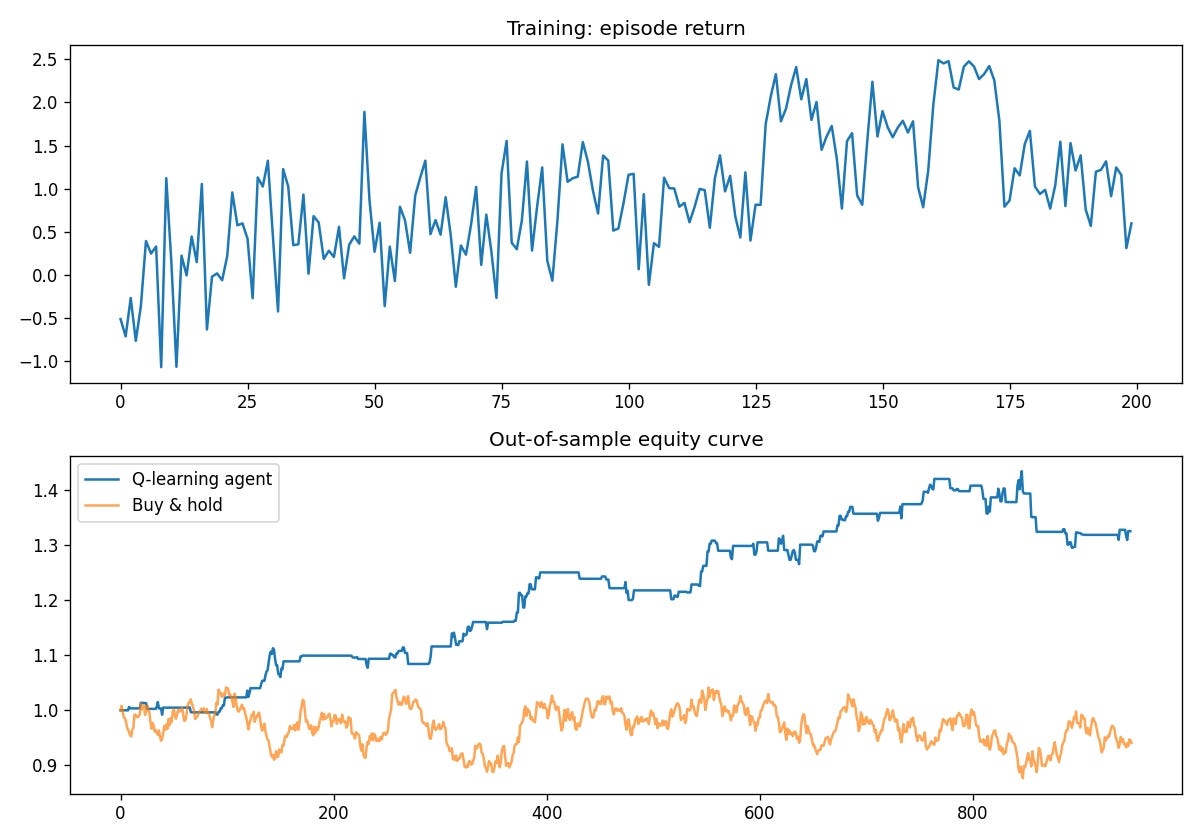
With the seed above, my run prints:
States visited      : 27
Test period return  : 32.51%
Buy & hold return   : -5.91%
Annualized Sharpe   : 1.02
Time in market      : 22.6%
Training episode returns rising as epsilon decays, and the out-of-sample equity curve beating buy & hold
Training episode returns rising as epsilon decays, and the out-of-sample equity curve beating buy & hold
Top panel: episode returns during training. Noisy and mostly negative early on while the agent explores at high ε, then improving as exploration decays and the Q-table converges. Bottom panel: the frozen policy on unseen test data, versus buy & hold. Keep this picture in mind for the comparison later.
Two things stand out. First, the agent is in the market only about a quarter of the time. It learned to wait for stretched z-scores rather than trade constantly, because the transaction-cost term punished churn. Second, you can inspect the Q-table yourself:
for (z_bucket, pos), q in sorted(agent.Q.items()):
    print(f"z-bucket{z_bucket}, pos{pos:+d} -> best action:{['flat','long','short'][int(np.argmax(q))]}")
Look at the extremes and the policy looks like something you’d design by hand. At the highest z-bucket the agent shorts, in the middle buckets it sits flat, and its overall behavior on the test set (fading stretched prices, waiting the rest of the time) is textbook mean reversion. Nobody told it the data was mean-reverting. It figured that out from reward alone.
Look closely, though, and you’ll also find entries that make no sense: a long in a high bucket, a short in a low one. These are rarely-visited states where the Q-values are still mostly noise. With only 200 episodes and a noisy reward, estimates for infrequent states never converge. This is an important point about RL in markets: the policy can be profitable overall while individual value estimates are garbage. Which is why you evaluate on out-of-sample P&L, not by inspecting the Q-table.
So that’s the real lesson of the exercise. When the environment has structure and the reward is well-designed, RL finds the structure. The obvious next question is what happens on real data, where the structure isn’t guaranteed.
Round 2: The same agent meets real Bitcoin
Synthetic data is rigged in the agent’s favor. So we ran the identical environment and agent, same state, same actions, same reward, on real data: 20,000 bars of BTC/USDT perpetual 15-minute candles from Bybit (late December 2025 through July 2026), fetched via ccxt. Chronological 75/25 split, so the agent trains on roughly December through May and gets tested on June and July, a stretch in which BTC fell about 10.6%.
Two changes for the real-data run, and both are worth adopting for anything you test on real markets.
First, ten seeds instead of one. A single RL run on noisy data is a coin flip. We train ten agents with different random seeds and report the distribution. (The full script, including the ccxt downloader so it’s one self-contained, copy-paste-runnable file, is in the appendix at the end of this post.)
Second, honest annualization and costs. Crypto trades 24/7, so the Sharpe uses √35,040 (that’s how many 15-minute bars fit in a year), not √252. Costs are 2 bps per position change, roughly Bybit’s maker fee.
Here’s what came back:
Symbol/timeframe : BTC/USDT:USDT 15m, cost=2.0 bps
Test period      : 2026-05-31 -> 2026-07-22
Buy & hold (test): -10.58%

 seed  return_pct  sharpe  time_in_mkt_pct  n_trades
    0       -5.71   -3.38             6.87       680
    1        0.00    0.00             0.00         0
    2        0.00    0.00             0.00         0
    ...      (seeds 2-9 identical: zero trades)

Seeds with positive return: 0/10
Seeds beating buy & hold : 10/10
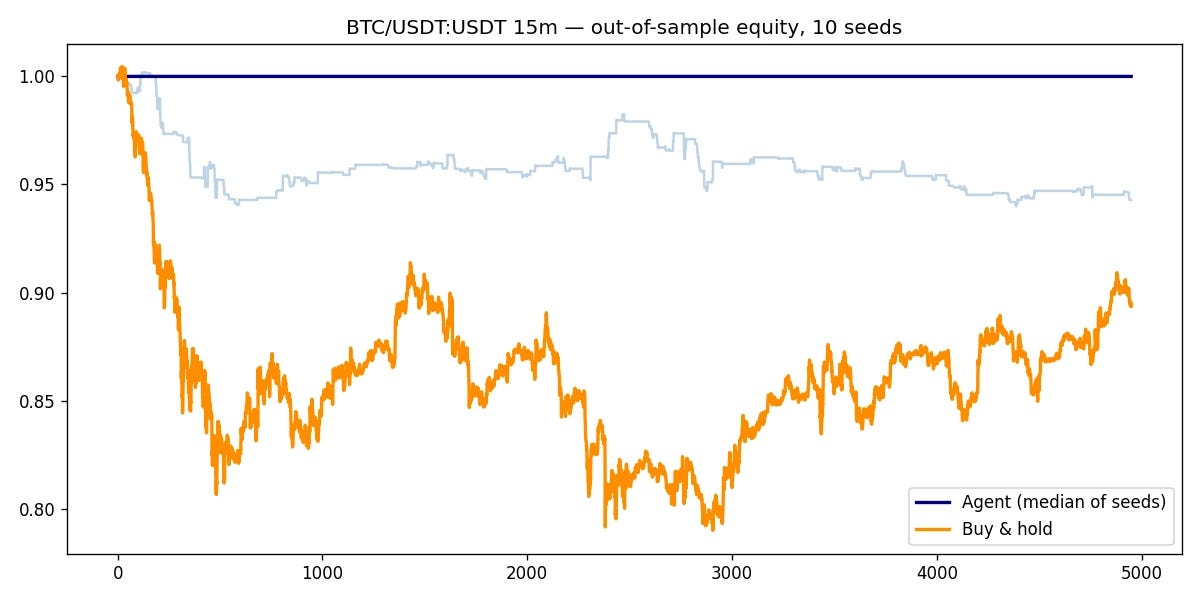
Out-of-sample equity curves: nine agents flat at 1.00, seed 0 drifting lower, buy & hold underwater throughout
Out-of-sample equity curves: nine agents flat at 1.00, seed 0 drifting lower, buy & hold underwater throughout
The whole experiment in one picture. The navy line at 1.00 is nine agents (and the median) doing nothing for seven weeks. The pale line drifting down to -5.7% is seed 0, the only agent that traded. The orange line is buy & hold, down as much as 20% at one point.
The main result: nine out of ten agents learned to never trade. Not “trade cautiously”. They placed zero trades across seven weeks of out-of-sample data. The tenth seed traded 680 times, was in the market 7% of the time, and lost 5.7%.
This is not a bug, and the agent is not broken. It’s the reward function doing exactly what we designed it to do. During training, the agent explored longs and shorts across every z-score bucket, and in expectation every one of them lost money after costs. The mean-reversion signal that was so profitable on our synthetic series simply isn’t exploitable at this frequency, in this form, on BTC. Flat pays a guaranteed reward of zero. Zero beats negative. Q-learning converged on abstention.
This is worth appreciating. A supervised model in the same situation would keep emitting predictions, because prediction is its only output. It has no way to say “pass”. The RL agent, because it optimizes decisions under costs, could say “there’s no edge here”, and it did. It arrived, from reward alone, at the oldest rule in trading: no edge, no position.
One more thing worth noting. Because the test period was a 10.6% drawdown for BTC, all ten agents outperformed buy and hold, including the nine that did nothing. Sitting in cash was the winning strategy. That “10/10 beat the market” stat is technically true but meaningless, and a good example of how backtest statistics can mislead. Always ask how a strategy won before celebrating that it did.
Seed 0 is the interesting one. The agent that thought it had found something traded its way to a -3.4 Sharpe. Across ten seeds, the only outcomes were “abstain” and “lose”. That’s the real market’s answer to our 27-state z-score agent.
Why this doesn’t (yet) print money, and why it mostly declined to try
Our agent succeeded on synthetic data because the game was rigged in its favor: the market was stationary and genuinely mean-reverting. On real BTC it correctly detected that neither holds, at least not in a form visible to a 27-state z-score policy. Before you conclude RL is hopeless, or start tuning hyperparameters until something “works”, four things are worth understanding.
Non-stationarity is the biggest problem. Our agent trained on December through May and was tested on June and July. Different regimes. Any pattern faint enough to need 300 training episodes to find is faint enough to vanish across that boundary. Practitioners deal with this through rolling retraining, regime features in the state, and walk-forward validation. Never a single train/test split, which we used here only for clarity.
RL needs a lot of data, and markets don’t have much. We gave the agent 300 replays of the same training window, but replaying the same seven months doesn’t create new information, and you can’t rerun markets with different random outcomes. This is a big reason tabular methods and simple state spaces often generalize better than deep RL here: fewer parameters, less to overfit. Our nine abstaining seeds are arguably tabular Q-learning’s small hypothesis space doing us a favor. A deep network might have hallucinated an edge instead.
The reward function is the strategy. The most important line in the whole experiment turned out to be the 2 bps cost term. It’s what turned “trade constantly on noise” into “don’t trade at all”. Rerun the BTC experiment with COST_BPS = 0and watch the agents churn thousands of trades. The abstention result is the cost model. Swap in a drawdown penalty, an inventory penalty, or a Sharpe-based reward, and each produces different behavior. In trading RL, most of your alpha-engineering effort goes into reward and state design, not the learning algorithm.
Backtest results are an upper bound. Even our result, honest as it is, is optimistic. We paid maker fees on every fill, with no slippage, no spread crossing, and instant execution at the close, and we ignored funding rates on the perpetual. Everything between an equity curve and live P&L moves in one direction: partial fills, slippage, funding, and your own overfitting across the experiments you didn’t publish. If a strategy barely works in a backtest, it doesn’t work.
Experiments worth running
The fastest way to learn is to break things on purpose, and the BTC result gives us better questions to ask:
Set
COST_BPS = 0on the BTC data. The agents will trade, a lot. Do any of them make money gross of costs? If yes, you’ve measured exactly how large your edge is and exactly why fees kill it. If no, the signal isn’t there even for free.Try 1h and 4h bars. Mean reversion and momentum live at different frequencies. Does the abstention verdict hold as you zoom out? Change
TIMEFRAMEand the annualization follows automatically.Try other symbols. Smaller-cap perpetuals are often less efficient than BTC. Same script, different
SYMBOL.Enrich the state. Add a volatility bucket, a longer-horizon z-score, or the funding rate. Notice how the Q-table grows and learning slows. This is the curse of dimensionality, and it’s the reason deep RL exists.
On the synthetic data, raise
cost_bpsto 5, then 20. Watch the agent’s time in market collapse toward the BTC outcome. Somewhere between “clean mean reversion at 1 bp” and “real BTC at 2 bps” is the entire story of quantitative trading.
Where we go from here
Everything in this post scales up along a well-marked path. The reset()/step() interface we used is the gymnasium standard, so wrapping this environment for stable-baselines3 and training a DQN or PPO agent is a small step. The table becomes a neural network, the states become continuous, and the pitfalls become sharper. From there, the natural directions are a richer state (volatility, funding, multiple horizons), a deep agent, and a serious walk-forward harness, to find out whether “don’t trade” survives as the answer once the agent can actually see more of the market.
Until then: run the code, break it, and remember what nine out of ten agents told us. Sometimes the strongest signal a model can give you is silence.
Happy trading,
Alex
Appendix: the full BTC script
Everything from Round 2 in one file: downloader, environment, agent, multi-seed runner, and plotting. pip install ccxt pandas numpy matplotlib tqdm, adjust DATA_DIR to wherever you keep data, and run it. It downloads fresh data on the first run and reuses the cached CSV afterwards, so you can iterate on the RL parameters without hammering the exchange.
"""
Q-learning on real BTC/USDT data from Bybit — all-in-one script.

Part 1: your ccxt downloader (unchanged logic)
Part 2: environment, agent, multi-seed train/evaluate

Run it directly:  python rl_trading_btc.py
It downloads fresh data unless USE_CACHED_CSV = True and the CSV already exists.

Dependencies: ccxt, pandas, numpy, matplotlib, tqdm
"""

import ccxt
import numpy as np
import pandas as pd
import matplotlib.pyplot as plt
from tqdm import tqdm
import time
import os
from datetime import datetime
from typing import Optional, Union

# ---------------------------------------------------------------
# 0. Config
# ---------------------------------------------------------------
SYMBOL = "BTC/USDT:USDT"
TIMEFRAME = "15m"        # used for both download and Sharpe annualization
NUM_BARS = 20_000        # ~7 months of 15m bars
DATA_DIR = "/Users/alex/Dev/ML/Data"
FILENAME = "BTC_USDT.csv"
USE_CACHED_CSV = True    # skip download if the CSV already exists

COST_BPS = 2.0           # per position change; ~Bybit maker. Try 5.5 (taker) too.
TRAIN_FRAC = 0.75        # chronological split
EPISODES = 300
N_SEEDS = 10             # distribution of results, not one lucky number

BARS_PER_YEAR = {
    "1m": 525_600, "5m": 105_120, "15m": 35_040, "30m": 17_520,
    "1h": 8_760, "4h": 2_190, "1d": 365,
}

# ---------------------------------------------------------------
# 1. Downloader (your code)
# ---------------------------------------------------------------
def download_ohlcv(
    symbol: str = "BTC/USDT:USDT",
    timeframe: str = "1m",
    num_bars: Optional[int] = None,
    until: Optional[Union[str, datetime]] = None,
    save_to_csv: bool = True,
    filename: Optional[str] = None
) -> pd.DataFrame:

    # Initialize exchange
    exchange = ccxt.bybit({
        'enableRateLimit': True,
        'options': {'defaultType': 'future'}
    })

    # Timeframe to minutes mapping
    timeframe_minutes = {
        '1m': 1, '3m': 3, '5m': 5, '15m': 15, '30m': 30,
        '1h': 60, '2h': 120, '4h': 240, '6h': 360, '12h': 720,
        '1d': 1440, '1w': 10080, '1M': 43200
    }

    if timeframe not in timeframe_minutes:
        raise ValueError(f"Unsupported timeframe: {timeframe}")

    minutes_per_bar = timeframe_minutes[timeframe]

    # Parse 'until' parameter if provided
    if until is not None:
        if isinstance(until, str):
            end_time = int(pd.to_datetime(until).timestamp() * 1000)
        elif isinstance(until, datetime):
            end_time = int(until.timestamp() * 1000)
        else:
            raise ValueError("until must be a string or datetime object")
    else:
        end_time = int(datetime.now().timestamp() * 1000)

    bars_needed = num_bars if num_bars else 1000
    max_bars_per_call = 1000
    chunks_needed = (bars_needed + max_bars_per_call - 1) // max_bars_per_call

    print(f"Downloading {symbol} {timeframe} data...")
    print(f"Target bars: {bars_needed:,} ({chunks_needed} chunks)")

    # Calculate the start time for the entire period
    total_minutes_back = bars_needed * minutes_per_bar
    start_time = end_time - (total_minutes_back * 60 * 1000)

    print(f"Start time: {pd.to_datetime(start_time, unit='ms')}")
    print(f"End time: {pd.to_datetime(end_time, unit='ms')}")

    all_ohlcv = []
    current_since = start_time
    request_count = 0

    try:
        for chunk in range(chunks_needed):
            bars_for_this_chunk = min(max_bars_per_call, bars_needed - len(all_ohlcv))

            request_count += 1
            print(f"Request {request_count}: Fetching {bars_for_this_chunk} bars from {pd.to_datetime(current_since, unit='ms')}")

            ohlcv_chunk = exchange.fetch_ohlcv(
                symbol, timeframe, since=current_since, limit=bars_for_this_chunk
            )

            if ohlcv_chunk:
                print(f"  Received {len(ohlcv_chunk)} bars")

                # Remove any overlapping data
                if all_ohlcv:
                    last_timestamp = all_ohlcv[-1][0]
                    ohlcv_chunk = [bar for bar in ohlcv_chunk if bar[0] > last_timestamp]
                    print(f"  After removing overlaps: {len(ohlcv_chunk)} new bars")

                all_ohlcv.extend(ohlcv_chunk)
                print(f"  Total bars collected: {len(all_ohlcv):,}")

                # Start the next chunk from the timestamp after the last received bar
                current_since = ohlcv_chunk[-1][0] + (minutes_per_bar * 60 * 1000)
            else:
                print(f"  No data received for chunk {chunk + 1}")
                # Move forward by the chunk size
                current_since += (bars_for_this_chunk * minutes_per_bar * 60 * 1000)

            # Break if we have enough data
            if len(all_ohlcv) >= bars_needed:
                print(f"Target reached: {len(all_ohlcv):,} bars")
                break

            # Add delay to avoid rate limits
            time.sleep(0.1)

    except ccxt.BaseError as e:
        print(f"Exchange error: {e}")
    except Exception as e:
        print(f"Error: {e}")
    finally:
        try:
            exchange.close()
        except:
            pass

    if not all_ohlcv:
        print("No data retrieved")
        return pd.DataFrame()

    # Sort by timestamp and remove any remaining duplicates
    all_ohlcv.sort(key=lambda x: x[0])
    unique_ohlcv = []
    seen_timestamps = set()

    for bar in all_ohlcv:
        if bar[0] not in seen_timestamps:
            unique_ohlcv.append(bar)
            seen_timestamps.add(bar[0])

    # Create DataFrame
    df = pd.DataFrame(unique_ohlcv, columns=['timestamp', 'open', 'high', 'low', 'close', 'volume'])
    df['datetime'] = pd.to_datetime(df['timestamp'], unit='ms')
    df.set_index('datetime', inplace=True)
    df.drop('timestamp', axis=1, inplace=True)

    # Trim to exact number if we got more than requested
    if len(df) > bars_needed:
        df = df.tail(bars_needed)

    print(f"\nDownload complete!")
    print(f"Total bars: {len(df):,}")
    print(f"Date range: {df.index.min()} to {df.index.max()}")

    if save_to_csv:
        if filename is None:
            symbol_clean = symbol.replace('/', '_').replace(':USDT', '')
            filename = f"{symbol_clean}_{timeframe}.csv"

        save_path = os.path.join(DATA_DIR, filename)
        os.makedirs(os.path.dirname(save_path), exist_ok=True)

        df.to_csv(save_path)
        print(f"Saved to: {filename}")

    return df

# ---------------------------------------------------------------
# 2. Environment
# ---------------------------------------------------------------
class TradingEnv:
    def __init__(self, prices, window=50, cost_bps=COST_BPS):
        self.prices = prices
        self.window = window
        self.cost = cost_bps / 10_000
        self.reset()

    def _zscore(self, t):
        w = self.prices[t - self.window:t]
        return (self.prices[t] - w.mean()) / (w.std() + 1e-9)

    def _bucket(self, z):
        edges = [-2, -1.5, -1, -0.5, 0.5, 1, 1.5, 2]
        return int(np.digitize(z, edges))

    def state(self):
        return (self._bucket(self._zscore(self.t)), self.position)

    def reset(self):
        self.t = self.window
        self.position = 0
        return self.state()

    def step(self, action):
        new_pos = {0: 0, 1: 1, 2: -1}[action]
        price_now, price_next = self.prices[self.t], self.prices[self.t + 1]
        pnl = new_pos * (price_next - price_now) / price_now
        reward = pnl - abs(new_pos - self.position) * self.cost
        self.position = new_pos
        self.t += 1
        done = self.t >= len(self.prices) - 1
        return self.state(), reward, done

# ---------------------------------------------------------------
# 3. Agent
# ---------------------------------------------------------------
class QAgent:
    def __init__(self, seed, n_actions=3, alpha=0.1, gamma=0.99,
                 eps=1.0, eps_min=0.05, eps_decay=0.98):
        self.rng = np.random.default_rng(seed)
        self.Q = {}
        self.n_actions = n_actions
        self.alpha, self.gamma = alpha, gamma
        self.eps, self.eps_min, self.eps_decay = eps, eps_min, eps_decay

    def q(self, s):
        if s not in self.Q:
            self.Q[s] = np.zeros(self.n_actions)
        return self.Q[s]

    def act(self, s, greedy=False):
        if not greedy and self.rng.random() < self.eps:
            return int(self.rng.integers(self.n_actions))
        return int(np.argmax(self.q(s)))

    def learn(self, s, a, r, s_next, done):
        target = r if done else r + self.gamma * self.q(s_next).max()
        self.q(s)[a] += self.alpha * (target - self.q(s)[a])

def train(agent, env, episodes=EPISODES, desc="training"):
    pbar = tqdm(range(episodes), desc=desc, unit="ep", leave=False)
    for _ in pbar:
        s, done, total = env.reset(), False, 0.0
        while not done:
            a = agent.act(s)
            s_next, r, done = env.step(a)
            agent.learn(s, a, r, s_next, done)
            s, total = s_next, total + r
        agent.eps = max(agent.eps_min, agent.eps * agent.eps_decay)
        pbar.set_postfix(eps=f"{agent.eps:.2f}", ep_ret=f"{total:+.3f}")

def evaluate(agent, env):
    s, done = env.reset(), False
    rewards, positions = [], []
    while not done:
        a = agent.act(s, greedy=True)
        s, r, done = env.step(a)
        rewards.append(r)
        positions.append(env.position)
    return np.array(rewards), np.array(positions)

# ---------------------------------------------------------------
# 4. Main: download (or load cache), then multi-seed run
# ---------------------------------------------------------------
if __name__ == "__main__":
    csv_path = os.path.join(DATA_DIR, FILENAME)

    if USE_CACHED_CSV and os.path.exists(csv_path):
        print(f"Loading cached data from {csv_path}")
        df = pd.read_csv(csv_path, index_col="datetime", parse_dates=True)
    else:
        df = download_ohlcv(
            symbol=SYMBOL,
            timeframe=TIMEFRAME,
            num_bars=NUM_BARS,
            save_to_csv=True,
            filename=FILENAME,
        )
        if df.empty:
            raise SystemExit("Download failed — no data to run on.")

    prices = df["close"].to_numpy(dtype=float)
    print(f"\nUsing {len(prices):,} bars: {df.index.min()} -> {df.index.max()}")

    split = int(len(prices) * TRAIN_FRAC)
    train_prices, test_prices = prices[:split], prices[split:]
    print(f"Train: {split:,} bars | Test: {len(prices) - split:,} bars "
          f"(test starts {df.index[split]})")

    ann = np.sqrt(BARS_PER_YEAR[TIMEFRAME])
    results, equity_curves = [], []

    seed_bar = tqdm(range(N_SEEDS), desc="seeds", unit="seed")
    for seed in seed_bar:
        agent = QAgent(seed)
        train(agent, TradingEnv(train_prices), desc=f"seed {seed} training")
        rewards, positions = evaluate(agent, TradingEnv(test_prices))

        equity = (1 + rewards).cumprod()
        sharpe = rewards.mean() / (rewards.std() + 1e-9) * ann
        n_trades = int(np.abs(np.diff(np.concatenate([[0], positions]))).sum())
        results.append({
            "seed": seed,
            "return_pct": (equity[-1] - 1) * 100,
            "sharpe": sharpe,
            "time_in_mkt_pct": (positions != 0).mean() * 100,
            "n_trades": n_trades,
        })
        equity_curves.append(equity)
        seed_bar.set_postfix(last_ret=f"{results[-1]['return_pct']:+.2f}%",
                             last_sharpe=f"{sharpe:.2f}")

    res = pd.DataFrame(results)
    w = TradingEnv(test_prices).window
    buy_hold = test_prices[w:] / test_prices[w]

    print("\n===== PASTE EVERYTHING BELOW THIS LINE BACK TO CHAT =====")
    print(f"Symbol/timeframe : {SYMBOL} {TIMEFRAME}, cost={COST_BPS} bps")
    print(f"Data range       : {df.index.min()} -> {df.index.max()} ({len(prices):,} bars)")
    print(f"Test period      : {df.index[split]} -> {df.index[-1]}")
    print(f"Buy & hold (test): {(buy_hold[-1] - 1) * 100:+.2f}%")
    print(res.round(2).to_string(index=False))
    print("\nAcross seeds:")
    print(f"  Return  : median {res.return_pct.median():+.2f}%  "
          f"(min {res.return_pct.min():+.2f}%, max {res.return_pct.max():+.2f}%)")
    print(f"  Sharpe  : median {res.sharpe.median():.2f}  "
          f"(min {res.sharpe.min():.2f}, max {res.sharpe.max():.2f})")
    print(f"  Seeds beating buy&hold: {(res.return_pct > (buy_hold[-1]-1)*100).sum()}/{N_SEEDS}")
    print(f"  Seeds with positive return: {(res.return_pct > 0).sum()}/{N_SEEDS}")
    print("===== END =====")

    fig, ax = plt.subplots(figsize=(10, 5))
    for eq in equity_curves:
        ax.plot(eq, color="steelblue", alpha=0.35)
    ax.plot(np.median(np.vstack(equity_curves), axis=0), color="navy",
            lw=2, label="Agent (median of seeds)")
    ax.plot(buy_hold, color="darkorange", lw=2, label="Buy & hold")
    ax.set_title(f"{SYMBOL} {TIMEFRAME} — out-of-sample equity, {N_SEEDS} seeds")
    ax.legend()
    plt.tight_layout()
    plt.savefig("btc_rl_results.png", dpi=120)
    print("Saved plot to btc_rl_results.png")
Both scripts in this post are complete and self-contained. The synthetic version needs only numpy and matplotlib, and the BTC pipeline in the appendix adds ccxt, pandas, and tqdm. Run them, rerun the experiments above, and post your results in the comments, especially if you find a configuration where the agents choose to trade and survive.
 |
|