Slippage: A Comprehensive Analysis and Non-Linear Modeling with Machine Learning

Slippage, the difference between the expected and actual execution price, is a critical component of trading execution analysis. It arises from factors such as order size, market liquidity, volatility, and market microstructure dynamics. Importantly, slippage exhibits non-linear behavior - for example, the market impact increases disproportionately with larger order sizes. Accurate modeling of slippage is therefore essential for building robust backtesting and trading systems.

By leveraging OHLCV data and advanced feature engineering, we aim to approximate institutional-grade slippage models without relying on order book or tick-level data. While a flat 0.01% slippage assumption is commonly applied across all trades, this oversimplification fails to capture the complexity of real-world execution costs. Optimizing trade execution with dynamic slippage insights can systematically reduce costs, particularly for strategies in less liquid or volatile markets.

The potential gains from using dynamic slippage models depend heavily on trading volume and market context. Even small improvements in slippage estimates - such as reducing slippage from 0.01% to 0.007% - can significantly enhance performance metrics like Sharpe Ratio, Information Ratio, and Alpha, especially for institutional strategies.

You can download code used in this analysis at: Slippage-Analysis.py

---

Key Components of Slippage

Market Impact

Large orders affect market prices by consuming liquidity across price levels. To quantify this effect, we often model price impact as a function of order size relative to market volume:

Here, $\alpha$, the impact exponent, typically ranges between 0.5 and 1, capturing the non-linear relationship between order size and market movement.

Liquidity Constraints

Liquidity plays a significant role in slippage. Metrics such as Amihud’s illiquidity measure, turnover, and volume ratios provide robust proxies for market liquidity:

Volatility Dynamics

High volatility amplifies slippage by increasing price uncertainty during execution, underscoring the importance of incorporating both historical and intraday volatility.

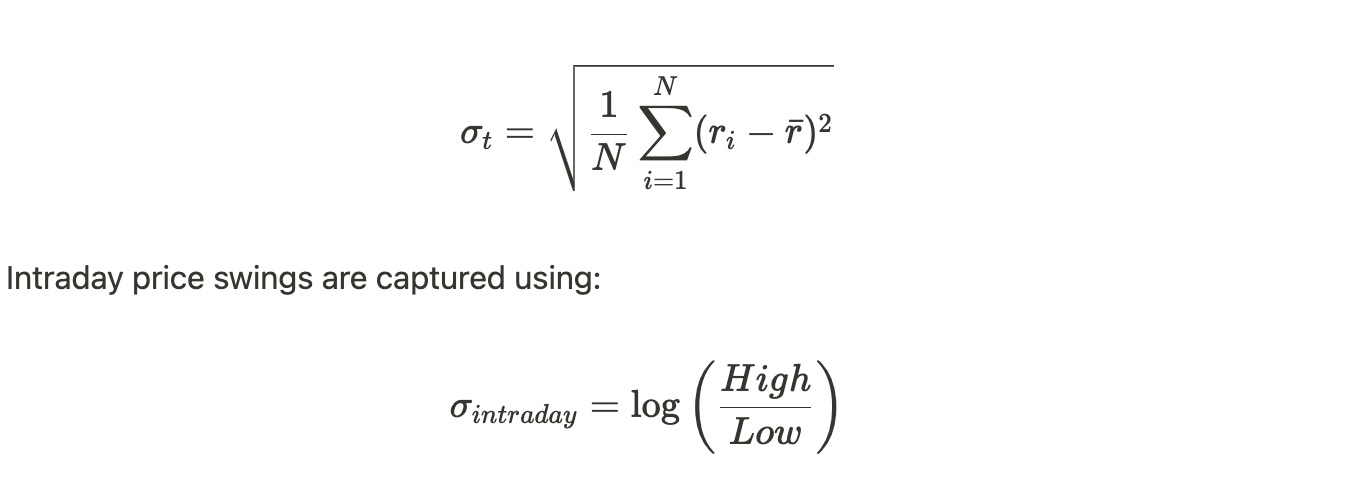
Please note that using just the high-low range neglects price clustering and noise, especially in illiquid or low-volume stocks, but here we make simple assumptions. One may use estimators such as Parkinson’s range-based volatility or Garman-Klass volatility, which are more robust for intraday data - and for which we have some posts in QuantJourney blog already.

Time of Execution

Time-of-day effects, such as opening or closing auctions, can significantly impact slippage due to temporary liquidity shifts.

Slippage Modeling: Methodology and Approach

To effectively model slippage, we focus on quantifying the relationship between observable market characteristics (e.g., price movement, volume, and volatility) and the unobservable execution inefficiencies caused by trading activity. Our modeling approach involves several key steps designed to capture the nuances of slippage dynamics.

• Data Availability - Given the absence of order book (Level 2/3) or tick-level data, our model relies on OHLCV (Open, High, Low, Close, Volume) data. This dataset provides accessible, aggregated market information while enabling robust feature engineering.

• Feature Engineering - Slippage is a multi-faceted phenomenon driven by market impact, liquidity constraints, and volatility dynamics. Through feature engineering, we transform raw OHLCV data into interpretable, high-quality predictors such as relative spread, volatility metrics, and liquidity proxies. This process enhances the model’s explanatory power.

• Non-Linear Relationships - Slippage is not linearly correlated with individual features (e.g., order size). To address this, we employ machine learning models capable of capturing non-linear relationships, such as Random Forest Regressors. These models are well-suited for high-dimensional data with complex interactions.

• Model Generalization - By using cross-validation (e.g., TimeSeriesSplit) during training, we ensure that the model generalizes well to unseen data, making it reliable for out-of-sample predictions.

This approach ensures that our slippage model is grounded in observable market patterns, even if direct trade data is unavailable.

With following analysis and regression code we find our objective for slippage analysis, and creating model for predicting slippage per set equities:

How the Model Works

The core modeling framework involves several steps:

1. Feature Preparation

Feature preparation is critical to reducing noise and creating predictors that reflect the underlying market dynamics:

• Liquidity Metrics: Features like Amihud Illiquidity and turnover measure the market's ability to absorb trades.

• Price Dynamics: Metrics like volatility, true range, and price acceleration highlight risk and momentum.

• Volume Metrics: Features like volume surge capture anomalies in trading activity.

See below feature preparation:

1.1. Price-Based Features

• Returns and Log Returns: These provide a foundational measure of price movement and are essential for calculating volatility and understanding price dynamics.

• Volatility Metrics (Short, Mid, Long): Different timeframes of volatility capture the market's risk over various horizons, which affects the expected slippage during trade execution.

• True Range: This measures the daily price range, accounting for gaps and providing insight into intraday volatility, which can impact slippage.

• Relative Spread: Serves as a proxy for the bid-ask spread when high-frequency data isn't available. A larger spread indicates lower liquidity and higher potential slippage.

• Price Acceleration: Identifies changes in momentum, helping to predict sudden price movements that could increase slippage.

• Range Intensity: Combines price range and volume to assess how trading activity affects price movements, indicating potential liquidity constraints.

Here is a code:

The following price-based features are computed to understand price dynamics:

1.2. Volume-Based Features

• Log Volume: Normalizes volume data, reducing skewness and highlighting significant changes in trading activity.

• Volume Moving Averages (Short, Mid, Long): Smooth out volume data over different periods, allowing for the detection of anomalies or trends in trading activity.

• Volume Ratios: Compare current volume to moving averages, highlighting periods of unusually high or low trading activity that could affect market impact and slippage.

• Volume Surge: Detects sudden spikes in volume, which could either provide liquidity (reducing slippage) or signal volatility (increasing slippage).

• Vol Impact: Models the non-linear relationship between order size and market volume, adjusting for the fact that larger orders have disproportionately higher impact.

And the code:

Volume-based features describe trading activity and liquidity:

1.3. Market Impact Features

• Amihud Illiquidity: Quantifies the price impact per unit of trading volume, directly relating to how much the price moves when trading a certain volume.

• Turnover and Turnover Volatility: Measures the overall trading activity and its variability, providing insight into market liquidity and stability.

• Base Impact and Impact Score: Calculate the expected market impact of a trade, adjusting for liquidity and volatility, essential for estimating slippage.

And the code:

1.4. Slippage Calculation

• Spread Cost: Represents the immediate cost of crossing the bid-ask spread, a fundamental component of slippage.

• Volatility Cost: Accounts for the risk of price movement during order execution, especially relevant in volatile markets.

• Market Impact: Estimates how the trade itself will move the market price, particularly important for larger orders relative to market volume.

• Momentum Cost: Incorporates the effect of price trends and momentum, acknowledging that trading against the trend can increase slippage.

• Liquidity Cost: Reflects the additional slippage due to illiquidity, as measured by the Amihud Illiquidity metric.

And the code:

Slippage is computed as a weighted sum of the following components: Spread Cost, Volatility Cost, Market Impact, Momentum Cost, and Liquidity Cost:

2. Model Selection

We use Random Forest Regressors for their ability to handle high-dimensional data and robustness against noise. This model is well suited for slippage modeling due to:

• Multicollinearity Handling: Random Forest effectively handles correlated predictors by randomly selecting a subset of features at each split, reducing the impact of multicollinearity.

• Non-Linearity and Interactions: The model captures complex, non-linear relationships between predictors (e.g., relative spread, volatility) and target slippage.

• Feature Importance: It provides a clear ranking of feature importance, enabling insights into the primary drivers of slippage.

Other potential models we tried: Gradient Boosting Regressors (e.g., XGBoost), but the results weren’t better.

To optimize our model, we use different hyperparameters such as max_depth,  n_estimators,  min_samples_split, and max_features via using randomized search, balancing model performance and generalization.

3. Cross-Validation

To ensure robust model evaluation and prevent data leakage, we have added TimeSeriesSplit, which is well know cross-validation technique designed for sequential data. This method works by creating training and validation sets that respect temporal order:

1. Setup: We used n_splits=5, creating progressively larger training sets while holding out future data for validation.

2. Rationale: By respecting the sequential nature of time-series data, TimeSeriesSplit mimics real-world trading scenarios where future data is unavailable during model training.

3. Trade-offs: Earlier splits have less training data, which could limit model performance. However, this trade-off ensures the model's reliability for out-of-sample predictions.

4. Model Regularization

To avoid overfitting, we constrain the Random Forest Regressor using:

• Limited tree depth (max_depth=4).

• Minimum sample sizes for splits and leaves (min_samples_split=30, min_samples_leaf=30).

• Feature subset selection (max_features="sqrt").

These settings balance the model's ability to learn complex patterns while maintaining generalizability.

5. Evaluation Metrics

The model is evaluated on:

• Mean Squared Error (MSE): Penalizes large prediction errors.

• Mean Absolute Error (MAE): Measures the average magnitude of prediction errors.

• R² Score: Quantifies the proportion of variance explained by the model.

• Cross-Validation R² (CV R²): Ensures out-of-sample reliability.

Results and Explanation

The model successfully identifies key drivers of slippage and accurately predicts slippage values in the test dataset. See some performance metrics:

• MSE: 0.000005 – indicating minimal large errors in prediction.

• MAE: 0.001393 – showing a low average prediction error.

• R² Score: 0.897689 – highlighting that 89.7% of slippage variability is explained by the model.

• CV R²: 0.768831 ± 0.125553 – suggesting consistent predictive power across time splits.

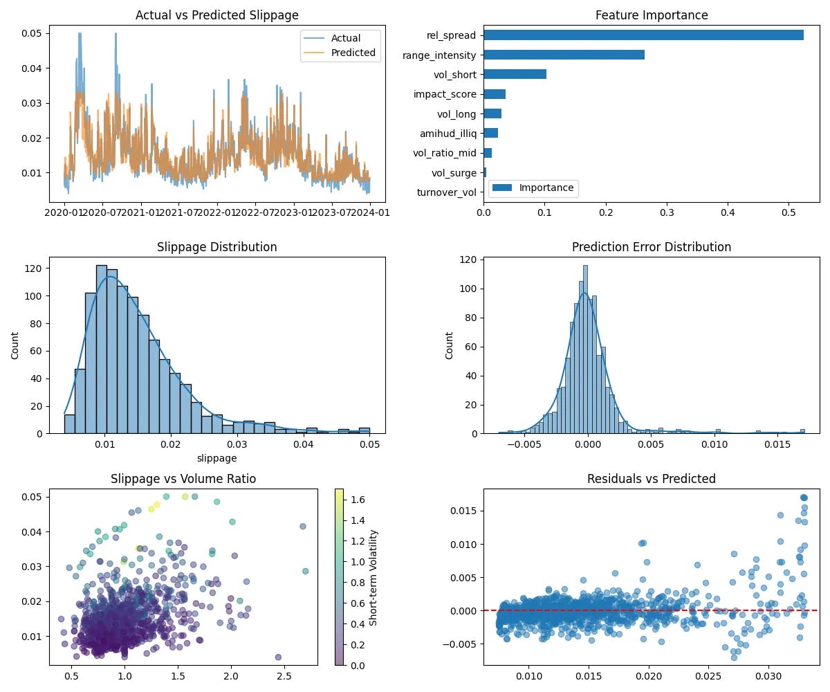
Feature Importance for slippage:

• Relative Spread (52.47%): A significant determinant, reflecting transaction costs' dependence on daily price range.

• Range Intensity (26.38%): Combines true range and volume, showing how price movement driven by liquidity impacts slippage.

• Volatility (10.30%): Indicates the role of short-term risk in execution inefficiencies.

• Impact Score (3.63%): Aggregates liquidity and volatility effects, emphasizing their combined influence on market impact.

Actual vs. Predicted Slippage

The Actual vs. Predicted Slippage plot shows:

• A strong match between actual and predicted slippage, indicating the model effectively captures slippage patterns.

• Slight underprediction in cases of very high slippage, suggesting there is room to improve the model for extreme scenarios.

Slippage vs. Relative Volume

The scatter plot reveals:

• Lower Slippage in Liquid Markets: Trades during periods of high relative volume generally experience less slippage due to better liquidity.

• Impact of Volatility: Even in liquid markets, higher volatility leads to increased slippage, showing the added uncertainty of price movements.

Feature Interpretability with SHAP

To better understand how individual features contribute to slippage predictions, we added SHapley Additive exPlanations (SHAP). SHAP provides a robust, game-theoretic approach to explain feature contributions at both global and individual prediction levels.

Global Insights: A SHAP summary plot ranks features by their average impact on the model's predictions.

Local Insights: SHAP dependence plots reveal how specific features influence predictions under different conditions, offering valuable granularity.

Integrating Slippage into Backtesting

To make our models actionable, we integrate them into our QuantJourney Backtesting framework with:

Dynamic Slippage Prediction: Predict slippage for each trade:

Conclusion

Slippage modeling bridges the gap between theoretical trading strategies and real-world execution. By combining advanced feature engineering, machine learning, and dynamic simulations, we’ve developed a framework that mirrors the practices of top hedge funds.

The focus isn’t just on building a model - it’s about ensuring it integrates seamlessly into the broader execution pipeline within QuantJourney Framework. This approach delivers actionable insights and robust risk management, which we apply for our research and trading flow.